WLM Response Time Distribution Reporting With RMF

(Originally posted 2013-03-20.)

If you’re running a workload with WLM Percentile Response Time goals take a look at the RMF Service Class Period Response Time Goal Attainment instrumentation. It’s in the Workload Activity Report but this post is about using the raw data to tell the story better than a single snapshot (or long-term “munging”) can.

(An example of a percentile response time goal is “90% of transactions must end in 0.2 seconds or less”.)

The raw data is in the SMF 72 Subtype 3 Response Time Distribution Data Section. For each Service Class Period an array of values is given: Each value represents a count of the number of transactions that ended within the response time constraints of that bucket. Here are some examples:

• Bucket 0 contains those transactions whose response time was less than 50% of the goal.
• Bucket 1 contains those that ended in more than 50% but less than 60% of the goal.
• The last but one bucket contains those that ended with a response time between 200% of the goal and 400% of it.
• the last bucket contains those that had a response time more than 400% of the goal.

I’ve omitted the middle buckets for brevity but note there’s one that’s up to 100% of the goal response time – a handy characteristic.

This “response time bucket” data is clearly a lot more use than just knowing the average response time achieved (or even the standard deviation).

My first implementation stacked up the buckets as percentages, and here’s an example:

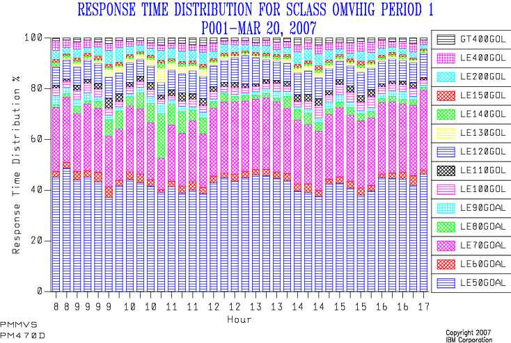
Isn’t it “busy”. 🙂 And what was the goal? And the legend is pretty cruddy, too. (This is explained by the reporting tool (SLR) insisting on using table column names as series names.)

Because I couldn’t see the wood for the trees I refurbished this graph a couple of years ago:

• The graph title states the goal.
• I only show the “within goal” and “not within goal” percentages. (Obviously I do this by summing up the appropriate buckets – and that’s where the “100% of goal” bucket boundary is needed.)

• When the goal is invariant I draw a datum line at the % number in the goal.
• I stopped letting SLR drive GDDM to create the graph and used the REXX GDDM interface to draw the graph instead. This meant I could label the series whatever I wanted, including using spaces. (This is considerably more fiddly programming – but I use the code on a frequent basis so that’s tolerable.)

The result looks like:

(This is actually from a customer performance test so don’t be put off by the repetitive hour labels on the x axis. One day I’ll get round to tidying up fractional hour labels – when I get sufficiently disgusted.) 🙂

This is much cleaner than the old version:

• For most of the time more than 90% of the transactions ended within the goal (0.5 seconds) – so the goal was met, sometimes comfortably.
• There were times when the goal was only just met.
• There was a protracted period when fewer than 90% of transactions ended quickly enough.

So, this has served me well for a while.

Thoughts For The Future

I think I might’ve gone too far in the direction of simplification with this: I’d like to add the “just made it” and “almost made it” buckets back in. (Whether I use shading or different colours for these is still up for debate.) The buckets I’m tempted to break out are 90% to 100% and 100% to 110%. The data I see, though, might drive me to use 80% to 100% and 100% to 120%. We’ll see.

I also can’t see how goal attainment relates to transaction rate:

• You might expect there to be a positive correlation though you’d hope for a neutral one.
• No correlation would mean something external was going on.
• Missing the goal for all transaction rates – “unsafe at any speed” 🙂 – is also significant: Either the goal is unrealistic or something that WLM can’t affect dominates response times.

So, adding a second y axis and plotting transaction rate against it would tell that part of the story.

I’d like to understand how the percentage of transactions ending in Period 1, Period 2, etc varies: Just today I had a situation where – over a weekend – the percentage of transactions ending in Period 1 dropped, as transactions got suddenly more CPU-heavy.

At present the code treats each Service Class Period independently, though it does print shift-average transaction rates ending in each period, along with the average CPU (not per transaction but totalled).

One thing I consider a very long stretch would be to make this a 3D chart – with the bucket boundaries considered to be “contour lines”. That would be very pretty 🙂 but hard to draw and even harder to explain: While I love pretty charts I actually want them to tell the story as clearly as possible.

Conclusions

I hope you’ll agree there’s lots you can usefully do with Response Time Distribution statistics. Most particularly If you have significant workloads with percentile goals – which would be almost 100% true for DDF, and true of quite a few CICS workloads.

I also hope you’ve found the evolution of a chart interesting: It’s been occasioned by lots of customer interactions over a number of years. I can’t say either of the two charts I’ve shown actually caused evolutions but I think them interesting examples.

We’ll see if I actually get to make the changes I’m contemplating: My hunch is I will – but I wouldn’t expect me to supply 3D glasses any time soon. 🙂