DDF Counts

(Originally posted 2016-01-17.)

I don’t think I’ve ever written very much about DDF. Now seems like a good time to start.

I say this because I’ve been working pretty intensively over the last couple of weeks on upgrading our DDF Analysis code. Hence the recent DFSORT post (DFSORT Tables).

I’m actually not the DB2 specialist in the team but, I’d claim, I know more about DB2 than many people who are. At least from a Performance perspective.

Actually this post isn’t about how to tune DDF. It’s about how to categorise and account for DDF usage. As usual I’m being curious about how DDF is used.

The Story So Far

A long time ago I realised it would be possible and valuable to “flatten” parts of the SMF 101 Accounting Trace record. A DDF 101 record is cut at every Commit or Abort – in principle.

And the DDF 101 record has additional sections of real value:

• QMDA Section (mapped by DSNDQMDA) has lots of classification information, most particularly detail on where requests are coming from.
• QLAC Section (mapped by DSNDQLAC) documents additional numbers such as rows transmitted.

In addition a field in the standard QWAC Section (mapped by DSNDQWAC) documents the WLM Service Class the work executed in. This field (QWACWLME) is only filled in for DDF.

So I wrote a DFSORT E15 exit to reformat the record so that all the useful DDF information is in fixed positions in the record. This makes it easy to write DFSORT and ICETOOL applications against the reformatted data. (In our code this data is stored reformatted on disk, one output record per input record.)

These reports concentrated on refining our view of what applications accessed DB2 via DDF. So, for example, noticing that the vast majority of the DDF CPU was used by a JDBC application (and its identity).

I also experimented with writing a DDF trace – using the time stamps from individual 101 records. Because installations can now consolidate DDF SMF 101 records[1] (typically to 10 commits per record) this code has issues. [2]

This code was good for “tourist information” but showed a lot of promise.

2015 Showed The Need For Change

A number of common themes showed the need for change, particularly in 2015.

There were some defects. The most notable was the fact that DB2 Version 10 widened a lot of the QWAC section fields. But also my original design of converting STCK values to Millisecond values was unhelpful, particularly when summing.

But these are minor problems compared to two big themes:

• Customers want to control DDF work better, particularly through better crafted WLM policies.
• Customers want to understand where the DDF-originated CPU is going, with a view to managing it down.[3]

These two themes occurred in several different customer engagements in 2015, but I addressed them using custom queries.

New Developments

So now in early 2016, while waiting for an expected study to start, I’m enhancing our DDF code. With the test data (from a real customer situation) the results are looking interesting and useful.

Time Of Day Analysis

My original code always broke out the SMF record’s date and time into separate TSDATE, TSHOUR, TSMIN, etc fields. This means I can create graphs by time of day with almost arbitrary precision.

My current prototype graphs with 1-minute granularity and (less usefully) with 1-hour granularity. And there are two main kinds of graph: Class 1 CPU and Commits.

With my test data (actually to be fed back to the customer) the Commits show an interesting phenomenon: Certain DDF applications have regular bursts of work, for example on 5 minute and 15 minute cycles. Normally I don’t see RMF data with 1-minute granularity so don’t see such patterns. Bursts of work are more problematic, including for WLM, than smooth arrivals. Now at least I see it.

What follows is an hour or so’s worth of data for a single DB2 subsystem, listing the top two Correlation IDs.

Here’s the Commits picture:

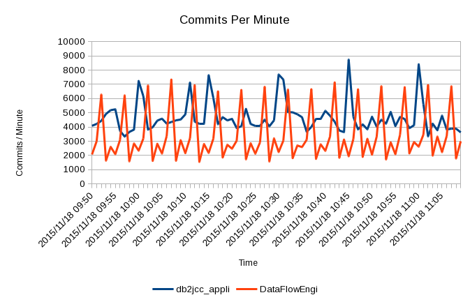
As you can see there are two main application styles [4], each with its own rhythm. These patterns are themselves composite and could be broken out further with the QMDA Section information, right down to originating machine and application.

And here’s the corresponding CPU picture:

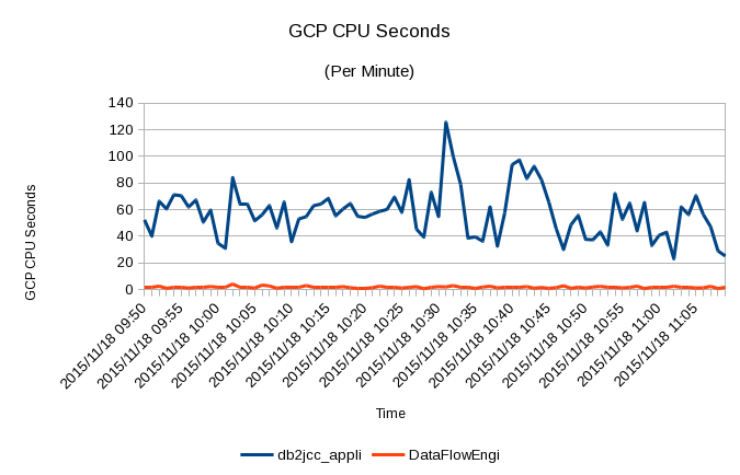
It shows the two applications behave quite differently, with the cycles largely absent. This suggests the spikes are very light in CPU terms and that other e.g. JDBC applications are far more CPU-intensive. Notice how the CPU usage peaks at 2 GCPs’ worth (120 seconds of CPU in 60 seconds). The underlying JDBC CPU usage is about 1 GCP’s worth.

zIIP

I’ve also added in three zIIP-related numbers:

• zIIP CPU
• zIIP-eligible CPU
• Records with no zIIP CPU in

zIIP CPU is exactly what it says it is: CPU time spent executing on a zIIP.

zIIP-eligible CPU has had a chequered history but now it’s OK. It’s CPU time that was eligible to be on a zIIP but ran on a General-Purpose Processor (GCP).

The third number warrants a little explanation: With the original implementation of DDF zIIP exploitation every thread was partially zIIP-eligible and partially GCP-only. More recently DB2 was changed so a thread is either entirely zIIP-eligible or entirely GCP-only. By looking at individual 101 records you can usually see this in action.

So I added a field that indicates whether the 101 record had any zIIP CPU or not – and I count these. Rolling up 101 records complicates this but my test data suggests the all-or-nothing works at the individual record level.

Workload Manager

Last year I did some 101 analysis to help a customer set up their WLM policy right for DDF.

Nowadays I get the WLM policy (in ISPF TLIB form) for every engagement.[5] So I can see how you’ve set up WLM for DDF. What’s interesting is how it actually plays out in practice.

And this is where the 101 data comes in:

• QWACWLME tells me which WLM Service Class a transaction runs in (only for DDF).
• The record has CPU data which enables you to calculate CPU Per Commit.
• You also get Elapsed Time Per Commit.

It would be wonderful if SMF 101 had the ending Service Class Period but it doesn’t. But at least you can do statistical analysis, particularly to see if the work is homogenous or not.

Similar statistical analysis can help you set realistic Response Time goals.

Here are a couple of graphs I made by teaching my code how to bucket response times and Class 1 TCB times, restricting the analysis to JDBC work coming into a single DB2 subsystem: [6]

Here’s the response time distribution graph:

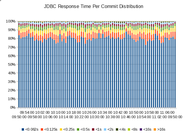
If this were a single-period Service Class one might suggest a goal of 95% in 0.5s – though if that were the case it’d be an unusually high value (0.5s).

You can also see attainment wasn’t that variable through this (75 minute) period.

And here’s the Class 1 TCB time distribution graph:

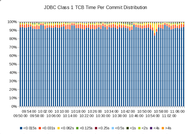
Notice how the bucket limits are lower than in the Response Time case. In my code I can fiddle with them separately.

Over 95% of the transactions complete using less than 15ms of CPU.

These two graphs aren’t wildly interesting in this case but they illustrate the sort of thing we’ll be able to see as analysts with the new code. I think it’s a nice advance.

In Conclusion

It’s been hard work and I’ve rewritten much of the reporting code. But I’m a long way forwards now.

It’s interesting to note the approach and, largely, the code is extensible to any transaction-like access to DB2. For example CICS/DB2 transactions. “Transaction-like” because much of the analysis requires frequent cutting of 101s. Most batch doesn’t look much like this.

I’d also encourage customers who have significant DDF work and collect 101 records to consider doing similar things to those in this post. This is indeed a rich seam to mine.

And I think I just might have enough material here for a conference presentation. Certainly a little too much for a blog post. 🙂

As always, I expect to learn from early experiences with the code. And to tweak and extend the code – probably as a result of this.

So expect more posts on DDF.