Bursty Batch – Small Reprise

In Bursty Batch I talked about how some customers have large amounts of batch work coming in all at once, and how a new WLM function in z/OS 3.1 might be handy in catering for it. And it subsequently occurred to me there is a cheap-to-collect and therefore almost universal method of assessing how bursty batch is. This post is about that method.

One section in SMF 70-1 is the ASID Data Area Section. It has system-level statistics for such things as the number of Started Tasks or TSO userids.

To take a relevant example, you can calculate the average number of batch address spaces by dividing field SMF70BTT by SMF70SAM.

So SMF70SAM is the number of RMF SMF 70 samples in an interval. Which makes SMF70BTT the total of all the sampled batch address spaces in the system. Hence the average. Samples in this context are one per second. So a typical 15-minute interval has 900 samples. We’ll come back to samples in a moment.

An average over 15 minutes is not a great determinant of burstiness. A lot can happen in that time. While one might drop the RMF interval to 5 minutes or even 1, most customers don’t run that way; The volume of RMF SMF records goes way up the shorter the interval. So this sort of interval length is good for benchmarks or Proofs Of Concept (POC’s) – of which I have data from one at the moment.

If an average is not good, it would be nice to compute a maximum. And this is where the neighbouring field to SMF70BTT comes in: SMF70BMM. This field is described in the SMF manual as the maximum number of batch address spaces. Actually, as happens occasionally, this description doesn’t entirely cover the ground. Let me explain why.

I said I’d return to samples, and here we are: The number of batch address spaces is sampled, once for each sample point. It is the maximum of these sampled values that SMF70BMM contains. But why do I make this point? It’s because the sampling process doesn’t rule out there being times – between the sample points – where the value was higher. So SMF70BMM isn’t a perfect measure. If you want perfect measurements you have to spend a lot more resources getting them.

But is SMF70BMM good enough? Take a look at the following graph.

Here I’ve plotted the maximum number of batch address spaces in the interval, and the average. This is real customer data, in case you wondered.

  • During the day the average number of batch jobs remains pretty constant, while the maximum varies wildly. You might discern an hourly pattern, with minor peaks on the half hour. This is interesting as it suggests work is thrown in on a timer pop of some sort. You’d have to examine SMF 30 to learn more about this.
  • At night there is more variation in the average, and much more in the maximum. The system peaks at over 60 jobs – according to SMF70BMM. Of course, this is a lower bound, but the picture is pretty clear.

From this pair of metrics we can learn a lot about the nature of batch in this system.

One thing we can’t learn that much about is balance between systems. The averages won’t show the fluctuations and the maxima can’t really be compared – as they might not coincide. In this case the average is the better of the two.

So, I think the SMF70BMM approach is valuable. It’s possible the other maxima – for, say, TSO or Started Tasks – is valuable. But I’d think rather less so.

The Making Of

Again I’m writing this on an aeroplane. It’s an Airbus A380 – in British Airways Economy. I make that point because, surprisingly to me, the seat pitch is adequate for a 12.9” iPad Pro.

And, if you were wondering about the title, in my head I misattributed it to Jimi Hendrix. In fact Queen and Paul Rodgers had a song called “Small”. And at the end of the”Cosmos Rocks” they had a song called “Small Reprise’. (You might prefer, though, Roger Taylor’s own “Small”.

I thought originally this post would indeed be a small reprise. In fact it’s quite lengthy. Oh well.

And the smudge on the graph is, of course, obfuscation.

In My Estimation

This post is about Coupling Facility sizing – particularly when you don’t have one to start with. And particularly CPU. (Memory is reasonably catered for with CFSizer – whether over the web or now in z/OSMF for z/OS 3.1.)

And the reason I’m writing about this is because I was recently asked to help size in just such a set of circumstances.

Narrowing The Doubt

Coupling Facility CPU usage is so variable that one is tempted to say “I’ve no idea” – but that isn’t a very satisfactory answer. So let’s see if we can do better. This is what I call “narrowing the doubt”.

  • When I was young the Country Capacity Planning Systems Engineer was reputed to be able to size a machine from the industry the customer was in and the number of employees. Those – late 1980’s – were simpler times. I would consider this the widest possible doubt short of “I’ve no idea”.

  • Narrower might be to see what other customers of a similar size have configured, along with how well it worked for them, as well as something about the workload.

  • Narrower still, perhaps, might be some guesses at request rates and service or Coupling Facility CPU times. We can establish reasonable numbers for the latter. Don’t quote me but 3 – 5μs for a lock structure and 10 – 20μs for a cache structure might be reasonable. There are two immediate problems with this:

    • These estimates are quite wide-ranging.
    • We don’t know the request rates.
  • Benchmarking can narrow the doubt further. But that’s a luxury few sites have available to them. Further, it might not reflect reality too closely.

  • Without benchmarking, or even with, a cautious approach to implementation is indicated. In this recent case there is a roughly 20% / 40% / 40% split. It makes sense to implement the 20% first, then one of the 40% ones, then the other. There are a couple of problems with this:

    • It might not be possible to implement this way.
    • The first or second portions might not be representative of the whole.

When it comes to “narrowing the doubt” it is as well to understand how wide the residual doubt actually is. If it remains – in your opinion – very wide you have to call that out. In a recent processor sizing situation I did just that. It might sound like defeatism but calling it out early allows people to plan for if the estimate is lower than the reality. In that case part of the reason for selecting a z16 A02 over a z14 ZR1 was the upgradability – in late 2023 – of the z16.

And the topic this post addresses has a lot of doubt. But I’ve tried to outline techniques for narrowing it. Of course there might be others.

Instrumentation

What I haven’t done so far is to describe the instrumentation that helps assess Coupling Facility CPU cost. There are two levels of this, both from SMF 74-4:

  • At the Coupling Facility level fields R744PBSY and R744PWAI can be used to compute CPU busy. This – for shared Coupling Facilities – might need to be augmented with SMF 70-1.
  • At the structure level field R744SETM gives you the CPU used in the Coupling Facility not the coupled z/OS. You have to sum up all the request rates from all the systems accessing the structure, whether synchronously or asynchronously. Then you can divide the R744SETM by this sum to compute a CPU-per-request number. The actual fields are too numerous to mention here.

But obviously, without an actual Parallel Sysplex or Datasharing (or whatever) environment there’s nothing to measure.

Conclusion

I should point out that you’d not want to run a Coupling Facility above, say, 50% busy. Pragmatically, you need to understand recovery scenarios – especially “white space”.

Further, you’d want to understand how structures scale with request rates. Tough to do if you don’t have any structures to start with.

The Making Of

This is one of a pair of blog posts drafted on the plane to Johannesburg. It did, however, get the benefit of several “sleep on its”, particularly the instrumentation section and the conclusion.

Bursty Batch

Bursty batch is quite common. For example, a customer I’m dealing with right now kicks off a burst of batch at 7PM and another burst at 10PM. I doubt that customer is reading this blog post. Another customer has a burst of batch kicking off at 2AM. They probably will read this post. But their operational security is assured: This is quite common. 😃

It’s worthwhile thinking about how this comes to be:

  • In the abovementioned cases there are business reasons for the release of batch at specific times. In their case instructions from external actors.
  • The ending for the day of a CICS service is another example – which might be a bounce to let batch run and then pick up new files.
  • Some prerequisite operation completes.
  • Some arbitrary definition of when the batch starts.

In any case a lot of work suddenly can run. But should it?

The temptation is to let it all in. Possibly motivated by the necessity to make it run as quickly as possible. But this is not consequence free: It can lead to thrashing.

CPI As An Indicator Of Thrashing

If we throw too much work in at once you might expect thrashing of CPU elements, such as the cache hierarchy.

This, for one, can lead to a typical instruction taking longer. I hope it’s obvious to you that cache misses cause CPU cycles while the data is fetched. Even cache hits serviced from another drawer can take a few hundred cycles. These are wasted cycles. Now, whether this leads to elongated run times is another matter. Suffice it to say an increase in CPU time for a job makes it more prone to queueing – which can lead to even more cache-related wasted cycles.

Wasted cycles might have a financial impact. With older software licencing schemes, based around the peak rolling four hour average GCP CPU, it’s quite common to see the batch driving the cost. And quite often soft capping is involved – which stands to elongate things further.

SMF 113 includes two useful counters – at the logical processor level: Instructions Executed and Cycles While Executing Instructions. These are in the Basic Counter Set and have been there since z10 (i.e. the beginning). So you certainly can perform the calculation: Cycles Per Instruction (CPI) is Cycles While Executing Instructions divided by Instructions Executed.

(Don’t quote me but) I’m seeing CPI typically in the 2 to 4 range. I say “don’t quote me” because it depends on a lot of things, including processor generation but also LPAR design and workload. In all the customers I’ve ever seen there’s been a daily cycle (pardon the pun) that CPI is observed to follow.

By the way, if the LPAR gets busy it might cause unparking of Vertical Low (VL) logical processors- and work running on those will almost certainly exhibit a higher CPI than Vertical High (VH) and Vertical Medium (VM) logical processors. Bursty work could well do that. Which sometime explains why I see spikes in CPI, usually at the same time each day.

SMF 113 is typically recorded on the 30-minute SMF interval. You’d think that is far too long to capture bursty batch. But note:

  • Severe burstiness would “move the needle” – even if there were, say, 15 minutes of it. Conversely, you might consider it not severe if there was little trace of it.
  • If you see – in SMF 113 – a spike in CPI you can bet the actual spike was much worse.

I wouldn’t recommend you drop the SMF interval, hoping to capture such things better. That’s the sort of thing you leave to SMF 98.

But CPI is not the only indicator. You might see lots of other evidence, such as:

  • CPU Queuing, or zIIP-on-CP. This would be at the service class period level – in SMF 72-3.
  • Locking, buffer pool misses, etc in Db2 Accounting Trace (SMF 101).
  • Unexplained variations in job and step elapsed time.
  • Initiation delays – in SMF 30 and 72-3. We’ll come back to this one.

Of course, this isn’t an exhaustive list.

Is WLM Too Slow?

We don’t want WLM to be in “nervous kitten mode”. Namely overreactive. On the other hand we don’t want it to be underreactive, either.

We want WLM to make the right decisions, with the right data, in a timely fashion.

The latter is the sticking point; WLM operates in a matter of seconds, but each change is only going to add a few initiators. This is a “smoothed response” – which is generally better than “nervous kitten”.

So an onrush of submitted batch can lead to initiator delays.

You could dispense with WLM-managed initiators altogether – and hope to manually get it right. And you could have an excess of initiators and watch your batch thrash.

Fortunately there is (soon going to be) another way. Read on.

z/OS 3.1 WLM AI Initiators

This new Artificial Intelligence (AI) function observes your batch and predicts when the work will spike. Before the spike it will nudge WLM towards adding initiators.

I rather like this function and the word “nudge” is doing the heavy lifting here: The AI adds Initiator Delay samples (R723CTDQ in RMF SMF 72-3). This happens ahead of the predicted spike. But the samples are only one factor in WLM’s decision to add more initiators. System conditions have to be taken into account, such as GCP and (as of z/OS 2.5) zIIP.

This design looks good because it minimises the risk of over-initiation causing thrashing. And it tells something WLM has no other way of knowing: When work is coming over the horizon. Such as our 7PM, 10PM, and 2AM spikes.

Fairly obviously, I hope, the work has to be broadly predictable. If there’s a sudden burst of work that is “out of phase” you can’t expect the AI to spot that.

WLM Knows Best – Or Does It?

WLM gets it’s information in a number of categories:

  • Classification rules
  • Goals in the Service Definition / Active Policy
  • Sampled workload attainment
  • System conditions

And now another:

  • AI

The last ones are automatic (with AI only being there if you set it up). The first two are worth talking about:

  • You need to make sure the right batch is classified to the right service class. For example TWS (or OPC to us old folks 😃) can place late-running work on the critical path in a (supposed) Critical Batch service class. But many installations are doing this manually.
  • The batch goals need to be right – both period durations and goal values.

A note on the word “supposed”: TWS will assign such work to a specific service class name. It’s up to you to make sure that really is an appropriate service class. And much of that is to do with the other point: Decent goals.

Parting Shorts

Well, that was a long post. I wanted to get two concepts across:

  • Over-initiation can cause thrashing and SMF 113 and 72-3 can illuminate that.
  • z/OS has a nice new (optional) function that can help with delayed initiation.

Some other parting sho(r)ts:

  • It’s ever more important to get WLM classification and goal setting right.
  • Consider the value and possibility of feeding in more judiciously. Your batch might even perform better.
  • When thinking about whether z/OS 3.1 WLM AI Initiators will eventually be able to help you, plan for the z/OS AI foundation work to enable it and any other Systems Management capabilities that might come along. It’s not trivial but it’s not perversely difficult either.

The Making Of

This post was written on a flight to Istanbul – and tidied up on the flight back. The purpose of the trip is to present z/OS 3.1 to a bunch of Turkish customers. And I met with a few of them. It’s been too long since I was last here – and we all know why. 😕 So I was very pleased to meet them again – and this very topic came up in each call. I suppose there’s a shiny new thing to talk about so inevitably it will come up. But, one shouldn’t be in a “hammer looking for a nail” situation.

I won’t claim any errors or insults are the result of cramped conditions – of course.

Seriously, a longish flight gives me time to think and write.

Tips For Debugging A DFSORT E15 Exit

I suppose I’d better tell you what an E15 exit is – else you might not read the rest of the post. 😀

DFSORT (and its competitor) allow you to send records to an exit routine. This happens as the very first thing for processing an individual record. This routine is called an “E15 routine”. There are two other, similar, exit points that happen later in record processing – “E35” and “E32”.

These tend to be written in assembler, though they could be written in COBOL. My personal use cases are satisfied by the former.

But why write an exit routine at all? There are several reasons. You might want:

  1. Record selection criteria that are diffe rent from what DFSORT can offer. For example, based on a field in a variable location.
  2. To extract fields that aren’t in fixed positions.
  3. Multiple records created from one input record (even if you coalesce them later).
  4. To format fields in a particular way that isn’t doable or easy with DFSORT.

The first two are quite similar, of course. And the first three are the main reasons I write E15 exits. Though I have used Reason 4 – to convert timestamps into multiple fields.

Now, how does the above apply to SMF? SMF, of course, is my prime data source. SMF records consist of sections, addressed by triplets. The triplet mechanism allows for variable numbers of sections of a given type.

The SMF format very often leads to fields in variable positions and the need to break a record into groups for further processing.

So, to do all this, I write assembler E15 exit routines.

In fact this is almost the only time I write assembler – so I need all the help I can get. 😃

Here’s another source of such help:

But let’s look at this another way: If I write an assembler exit routine and wrap it in DFSORT I get my I/O done for free. No more mucking with BSAM, QSAM or VSAM. Plus I get other “slice and dice” for free. So I’m highly likely to write the bulk of my assembler code as a DFSORT exit routine.

Some Useful Tips

As the title suggests, this post is about debugging techniques so here are some. They’re things I actually used in my most recent debugging session. I think they’re useful.

Do A COPY First

Build up your DFSORT application in stages, starting with a COPY:

       OPTION COPY

This actually overrides eg SORT.

Once you’ve got the E15 exit working with COPY you can add in other elements, such as SORT, SUM, OUTFIL. Actually it’s as well to get the exit working with COPY before you add in INREC as well.

In general start at the beginning – the E15 exit – and work your way forwards, adding statements and refining them.

Stop After 1 Record To Begin With

It’s useful and quick to run with only 1 record being produced. In particular to make sure you can write a basic record.

       OPTION STOPAFT=1

You can always write a small number of records – and this is diagnostically different from writing just 1:

       OPTION STOPAFT=nnnn

I say that because the ability to loop over eg SMF sections in the input record isn’t trivial.

If you have a troublesome input record you might be able to avoid processing it – for now – with a combination of STOPAFT and SKIPREC:

       OPTION SKIPREC=nnnn,STOPAFT=nnnn+1

Actually, this isn’t one I had to use this time but I have in the past.

Write Diagnostic Data Into Output Records

You can write anything you like into the record the E15 exit routine passes back to DFSORT. I, for example, wrote some register values into the record my code passed back. I did, of course, delete that debugging code once I’d got over the problem I was trying to solve.

It needn’t be registers, of course. It could be contents of storage areas.

Forcing An Abend Can Help

If you want to see the state of play at any point you can force an ABEND. Coding

       ABEND 1

will get you an ABEND. But see below.

Code A SYSUDUMP DD

If you don’t you’ll get a SORTSNAP dump if the exit routine ABENDs which is rather short and doesn’t contain the input record nor any reformatted one, nor any other storage areas you might’ve GETMAINed.

If you do code a SYSUDUMP DD you’ll get a full dump. This is nice because:

  • Doing a find for “RTM2WA” will get you to the registers at the time of the ABEND.
  • You can see the address of the failing instruction and its offset into the exit load module.
  • You can navigate to storage areas, such as the input record and any reformatted output record.

Maintain A DFSORT Symbols Convention

Always code a SYMNAMES input DD and SYMNOUT output DD.

And here’s the convention I’ve used:

  1. Map the input record using symbols that don’t start with an underscore.
  2. If you have an INREC then map the record that results from it with symbols that start with an underscore.
  3. If you additionally have an OUTREC then use a double underscore for the results of that.

And so on.

GETMAIN Your Working Storage

If you use working storage then GETMAIN it and hang the address off the user exit constant.

Storing into the instruction stream is not performant and this technique minimises that.

Of course you can use DSECTs to map such storage areas – as I do.

Write To The SPOOL

Early on write the output data (probably SORTOUT DD at this stage) to the SPOOL. But don’t flood the SPOOL so restrict this to when you’re e.g. using STOPAFT.

This is a minor hint but it saves you flipping between ISPF 3.4 and SDSF to check both output aspects of the run:

  • The output data
  • Messages and Symbols information

Conclusion

That’s quite a kitbag of techniques. I will say that many of them have nothing to do with E15 exits or assembler; They make sense when developing any DFSORT application.


Behind The Scenes

If you’re going to write a blog post about debugging it’s advisable to do it as close to when you learnt the tips as possible. In fact most of the material for this post came from a mammoth debugging session this week – for SMF Type 74 Subtype 4. Still better would’ve been to have written it as I debugged – but the idea for the post emerged only during the session.

Then, a few days later, I decided it’d be a good idea to explain why you’d even want to write an E15 exit. It’s not good enough to say “if you know you know”.

Then again, another debugging session for a different SMF record (Type 30) a week later yielded a different tip.

And a pickiness point: I’ve tried to use the terms “exit point” and “exit routine” correctly. Generally one just says “exit” for both but I think that less clear.

z16 ICA-SR Structure Service Times

It was recently brought to my attention that CFLEVEL 25, made available with IBM z16, improved ICA-SR links.

(I don’t know why I didn’t spot this before – but it’s documented in several places, including IBM Db2 13 for z/OS Performance Topics, an interesting Redbook. (I actually read this from cover to cover during a recent power outage.)

An ICA-SR link is short distance, and faster than CE-LR (long reach) links. The ICA-SR fanout connects directly to the processor drawer. There are two flavours:

  • ICA-SR (Feature Code 0172)
  • ICA-SR 1.1 (Feature Code 0176)

You can carry both of these forward into a z16. This post, though, is exclusively about ICA-SR 1.1.

Note: ICA-SR links can be up to 150m. Any longer and you’d be using CE-LR links.

What’s Changed

The ICA-SR 1.1 hardware didn’t change between IBM z15 and z16. What changed is the protocol.

To quote from IBM z16 (3931) Technical Guide

On IBM z16, the enhanced ICA-SR coupling link protocol provides up to 10% improvement for read requests and lock requests, and up to 25% for write requests and duplexed write requests, compared to CF service times on IBM z15 systems. The improved CF service times for CF requests can translate into better Parallel Sysplex coupling efficiency; therefore, the software costs can be reduced for the attached z/OS images in the Parallel Sysplex.

The changes that lead to these improvements are:

  1. Removing the memory round trip to retrieve message command blocks.
  2. Removing the cross-fiber handshake to send data for a CF write command.

It almost doesn’t matter what the changes were – except Item 2 probably explains the relatively large improvement for write requests (whether duplexed or not).

Impact Of The Improvement

So, how do we interpret the effect of these improvements? Usually we divide structure service time decreases into two areas of benefit:

  1. Workload response time decreases and throughput improvements.
  2. Coupled CPU reductions for synchronous requests.

(Conversely, an increase in service times leads to the opposite effects. This would typically be a matter of increasing distance.)

On the first point, most applications aren’t overly sensitive to coupling facility request times. Often they’re more sensitive to other aspects, such as obtaining locks or buffer pool invalidations. But one shouldn’t dismiss this out of hand.

On the second point, recall that a coupled (z/OS) processor spins waiting for a synchronous request. So, the faster a synchronous request is serviced the lower the z/OS CPU cost.

It’s worth noting that individual processors are faster on a z16 compared to a z15. So it might be that the z16 ICA-SR 1.1 improvements more or less match the coupled engine speed improvement. You might consider this “running to stand still” but both improvements are net gains for most customers. Further, it makes ICA-SR 1.1 more attractive on a z16 than ICA-SR.

A reduction in request service times over physical links might make using external coupling facilities more feasible. This could open up more architectural choices – such as using external coupling facilities where today you use internal.

Note: A reduction in service times can lead to some formerly asynchronous requests becoming synchronous. This is not a request-level conversion process but rather a consequence of the dynamic conversion heuristic; Now more requests are serviced quicker than the heuristic’s thresholds. If this happens the coupled (z/OS) CPU might well go up. Of course former async requests would probably have even lower service times – because they’d become sync.

Conclusion

It seems appropriate to encourage anyone moving to z16 to ensure their ICA-SR links are 1.1 – whether they brought them forward or perhaps replaced older ICA-SR links. Of course, there might be a cost downside to balance against the upsides.

It also seems to me to make ICA-SR on z16 more attractive, relative to IC links on previous generations. That might increase configuration options, including adding more resilient design possibilities.

Two other RMF-related things to note:

  • RMF doesn’t distinguish between ICA-SR generations; They all have Channel Path Acronym “CS5”. (CE-LR is “CL5” and IC Peer is “ICP” – for completeness.)
  • RMF doesn’t have a fine-grained view of Coupling Facility request types. (It does know about castouts but that’s about all.)

Neither of these is RMF’s fault; It’s able to report only based on the interfaces it’s using.

One final thought: As articulated in A Very Interesting Graph – 4 months ago – there’s much more to request performance than just ICA-SR niceties. But the improvement in z16 ICA-SR 1.1 is surely welcome.

Mainframe Performance Topics Podcast Episode 33 “These Boots Were Made”

I hope you can tell that Marna and I had a lot of fun making this episode.

I can’t recall which of us came up with the cultural reference. But it sort of developed – until the aftershow was sort of inevitable.

Anyhow here are the show notes for Episode 33. The podcast series is here and on all good podcasting services.

Episode 33 “These Boots Were Made” long show notes.

This episode is about our Mainframe Topic.

Since our last episode, Martin was at the Munich Z Resiliency Conference, and IntelliMagic zAcademy Where Are All The Performance Analysts? – A Mainframe Roundtable.

What’s New

  • Preliminary 3.1 upgrade materials can be found in APAR OA63269 . Another APAR will be done closer to GA.

  • Python 3.11 zIIP enablement, for certain modules only, up to 70%. This is available back to z/OS V2.4 with APAR OA63406 and PH52983.

Mainframe – z/OS Validated Boot

  • This function is only on latest hardware and software: z/OS V2.5 or later, IBM z16 A01 or A02 May 2023 microcode level and another follow-on level.

  • The point is to ensure IPLs are from known, unmodified, validated in-scope artefacts, so that you can initiate a system with known objects. This is needed for Common Criteria Evaluation.

  • Good for an organisation concerned about security.

  • Two pieces to the solution: Front end and back end.

  1. Front-End first:

    • Sign in-scope IPL time artefacts, done by the customer with their own private key.

      • You could choose to do this at an initial product install: Eg z/OS 2.5 -> 3.1. Note that z/OSMF workflows delivered with ServerPac can help.

      • Note z/OS V2.5 is requirement for driving system.

      • Also you would need to do this signing post-PTF installation, as applying PTFs leads to artifacts becoming unsigned.

      • You can sign now and validate later, as this portion does not have a requirement on the IBM z16 HW.

      • The Certificate you signed with, needs to be exported (via RACF, for instance), which will have the public key in it.

      • The in-scope artifacts that must be signed for z/OS Validated Boot is: IPL text, nucleus, standalone dump text, LPA.

      • A helpful utility IEAVBPRT can be used to report on what in a data set has been signed or not. Use this as possibly a best practice after applying maintenance, before IPL with Audit.

  2. Now Back-End:

    • Signatures validated during IPL time , and this is when you have the IBM z16 HW requirement. You must import the certificate (from the Front-End) into the IBM z16 HMC.

    • IPL time has additional requirements:

      • IPL with CLPA. CLPA is building the Link Pack Areas in virtual memory. CLPA enforced for Validated Boot IPL.

      • LPAR has to have Virtual Flash Memory. Specific requirement for Validated Boot is to allow PLPA to page to somewhere secure. You might have other users of VFM, so size for both. Probably other users are much larger.

    • You have a choice of IPL type: CCW and List Directed.

      • Channel Command Word (CCW) has been around forever. A CCW IPL is compatible with signed load modules.

      • List Directed (LD) is new. This type of IPL does signature validation in two modes: Audit and Enforce.

        • Audit is used just for reporting.

        • Enforce is used for validation and potential failure. Failure is one of a few wait states with a message. Wait state indicates the first problem.

      • Do an Audit first, fix any problems, then do Enforce. Go round the loop when applying maintenance.

  • You need to revise IPL procedures, in particular deciding when to do Audit versus Enforce. Reminder: Maintenance would bias you towards Audit followed by Enforce. Be careful when selecting mode for an emergency IPL.

Performance – Db2 Open Data Sets

  • Follows on from Episode 32 Performance Topic – which we’ll call Part 1. This time we don’t have Scott Ballentine with us. Recall he’s a z/OS developer and here in Part 2 we’re concentrating on Db2.

  • In Part 1 we were talking about physical Open and Close. That is Open data sets as z/OS would see it.

  • Db2 has an additional notion of logically Open and Closed data sets. We’ll discuss both in this follow up topic. And try to keep them straight.

Physical Open And Close

  • If a data set is needed – for the portion of an index space or table space – the Db2 transaction will experience a delay if the underlying data set is physically closed. To minimise this Db2 uses a deferred close process – keeping data sets open beyond end of use. It also minimises the CPU used for opening and closing data sets by keeping a pool of them open.

  • Of course, as mentioned in Part 1, a lot of this is about managing the virtual storage for the open data sets

  • The DSMAX Db2 subsystem parameter was mentioned in Part 1. It controls the number of physically open data sets for the subsystem. When DSMAX is approached Db2 starts physically closing data sets. First, page sets or objects that are defined with the CLOSE YES option are closed. The least recently used page sets are closed first. When more data sets must be closed, Db2 next closes page sets or partitions for objects that are defined with the CLOSE NO option. The least recently used CLOSE NO data sets are closed first.

  • Db2 Statistics Trace documents the number of open data sets and the open and close activity. So you can see if your DSMAX is set sufficiently high. But, as we saw in Part 1, virtual storage comes into play and ultimately limits what a safe DSMAX value would be.

  • Two recent APARs are of interest: PH33238 and PH27493. In addition to the CLOSE YES vs CLOSE NO distinction, Data sets opened exclusively for Utility access will be pre-emptively closed after 10 minutes and will be at the front of the queue to be closed when DSMAX is approached. Fixes for both APARs are required for this to work right.

Logical Open And Close

  • Usually known as Pseudoclose – is a switch from R/W to R/O. It’s not a physical close at all.

  • Its main role is to manage inter-Db2 read/write interest, for Datasharing efficiency purposes; It’s expensive to go in and out of Group Buffer Pool (GBP) dependency.

  • When there is at least one updater and maybe one reader there is read/write interest and Db2 has to do more work in Datasharing. While flipping in and out of Inter-Db2 read/write is not a great idea there is an efficiency gain in dropping out of this state judiciously.

  • Two Db2 subsystem parameters have traditionally been used to control pseudoclose: PCLOSET and PCLOSEN. “T” for Time and “N” for number of checkpoints. PCLOSEN is gone in V12 with APAR PH28280, as part of a DSNZPARM simplification effort. (DSNZPARM is the general term for subsystem-level parameters.) So PCLOSET would need adjusting down to whatever mimics PCLOSEN – in anticipation of this APAR or V13.

  • Sidebar: Putting Db2 maintenance on is an inevitability. Another example if this is the changed Db2 DDF High Performance DBATs’ behaviour.

Open Data Set Conclusion

  • So we have two different concepts for Db2: Physical open & close. And logical open and close aka Pseudoclose.

  • And you’ll note the interplay – at least for physical open and close – between z/OS and Db2. Hence the Part 1 – primarily z/OS. And this Part 2 – primarily Db2.

Topics – Messing With Digital Electronics

  • Martin had discussed his various Raspberry Pi efforts, mainly for software. But note he uses breadboards for his electronics projects as his soldering has become atrocious.

  • Martin has used various commercial input devices before:

    • Streamdecks (lots of them!). Started off with 6 button Mini. Then 15 button Stream Deck, then 32 button XL.

      • Now Stream Deck Plus, with 4 knobs and only 8 buttons.

      • But he doesn’t have the Stream Deck Pedal – so not playing with a full deck. 😀

    • Xencelabs Quick Keys. This is portable, with only one knob.

  • All rather expensive, but at this point a sunk cost, and is most of what he uses “In Production”.

  • But then there was interest in building his own input devices.

    • Some things he’s not interested in building his own: keyboards, mice, touch screens and voice assistants. (There is a community of people who do like to build their own keyboards.)

    • However, interested in other things that trigger actions. Action which might be simple, or might be complex, automations.

  • At Christmas, got a Pi Hut Maker Advent Calendar, which was pretty cheap.

    • 12 projects, one per day. From very simple to quite complex, driven by Raspberry Pi Pico.

      • Raspberry Pi Pico is not a computer – like Pi. It is a microcontroller

      • Microcontroller has a runtime but no operating system that we’d recognise

      • You load in a Micropython or CircuitPython interpreter or you standalone C program

      • Pico W is a wifi variant – and highly recommended as it’s only slightly more expensive than the non-wifi variant.

    • Lots of digital and analogue inputs and outputs, and under $10.

  • Then Martin bought a Pico W. which was also under $10. It has Wifi, and now has Bluetooth support. Still no soldering required – as he buys the “H” (pre-soldered headers) variant.

  • First actual project – with Pico W

    • RFID cards kick off automations. Tap on RFID detector with credit card sized card. Actual credit cards usually work.

      • On iOS with Shortcuts via Pushcut. Creates a new Drafts draft with a date and time stamp for meeting notes

      • On Mac OS via Keyboard Maestro. This automation opens apps and arranges them on his second screen.

      • Both these are Swiss Army knife affairs for building automations. Above automations were just a proof of concept – but they are used regularly as they have inherent value to Martin.

  • Second project – with Pico W

    • Using Rotary Encoders, otherwise known as twirly knobs, but not the same as a potentiometer or “pot”.

    • They’re good for adjusting things like font sizes – as opposed to push buttons, which aren’t.

    • Difficult to program but there are samples on the web. Martin only did this project to prove it could work.

    • There was a lesson in the importance of physical considerations: He had some trouble fitting into a plastic case he bought – because of the clearance above the Pico W and below the rotary encoders.

  • Third project – with Adafruit Macropad

    • It’s a kit comprising a Pico plus light up keypad plus small status screen plus a twirly knob. It acts as a Human Interface Device (HID). (The USB standard divides devices into mass storage devices and human interface devices, plus more obscure device classes.)

    • Uses CircuitPython – as that has HID support and MicroPython doesn’t yet. (It’s not difficult to convert code between these two python variants.)

    • Automated a bunch of functions of his personal Mac Studio. With his programming each key lights up when pressed, and the small OLED screen says what the function is.

    • At present the twirly knob just moves the text cursor in his text editor. (BBEdit and Sublime Text but any text field would work the same.)

  • Most of the projects were just for fun, and there was a lot of fun in it.

    • Some practical stuff: Text automation, RFID to kick off stuff, e.g. a “good morning” routine.

    • There is lots of potential for practical applications, and as a hobby it’s pretty cheap. So is open source software. And the field is evolving fast. For example, Pico W just got Bluetooth support without new hardware.

Out and about

  • Marna will be at SHARE New Orleans,the week of August 14th, and is waiting to hear about IBM TechXchange week of September 11, 2023.

  • Martin (and Marna) will be at the GSE UK Annual Conference – Oct 30th – Nov 2nd, 2023.

On the blog

So It Goes

Reporting For Duty?

I’m writing this on a flight to Munich, where I’m presenting Parallel Sysplex Resiliency at a customer conference. By the way I wonder what happened to the word “resilience” and what the difference is between that and “resiliency”. But, it’s a trip to a nice city and I expect to run into lots of friends there. And I’m looking forward to presenting.

In this post I want to discuss report classes. In particular the approach one might take to defining them.

Report Classes Are Cheap And Abundant

Unlike with service classes, you can have practically as many as you like. There is no discernible cost to having more. Except for one thing that is, I hope you’ll agree, an upside: Just as RMF will report service class period attainment, so too with report classes. So you get more SMF data written – but it is valuable data.

Most customers are collecting SMF 72-3 so there’s nothing to do to get report class data – except define some report classes. (The mechanics of doing so, whether using z/OSMF or ISPF panels, is beyond the scope of this post.)

One other thing on cheapness: SMF 72-3 is much cheaper to collect and store than SMF 30 address space data. And can in many aspects perform the same role. Which is a key advantage.

So, if they’re so good let’s think about defining some.

Coverage

One thing I like to see is all the work in a system having a report class defined. From an instrumentation point of view it’s a second coverage of the work, alongside report classes. All work has a service class but not all work has to have a report class. But ideally it should. Hence my use of the term “coverage”.

All CPU that can be fairly associated with a service class is. Of course, not all can. Hence the existence of “uncaptured time” from which one can compute a “capture ratio”. This applies to both general purpose CPU (GCP) and zIIP.

A more interesting case, though, is memory. So let’s use it as our measure of coverage – at least for the purposes of this post.

We define memory usage by a report class or service class as SMF 72-3 field R723CPRS divided by the summarisation interval. (If you do this for a period longer than the interval you will need to sum the denominator and the numerator before dividing.) There is some adjustment required to turn the result into MB or GB.

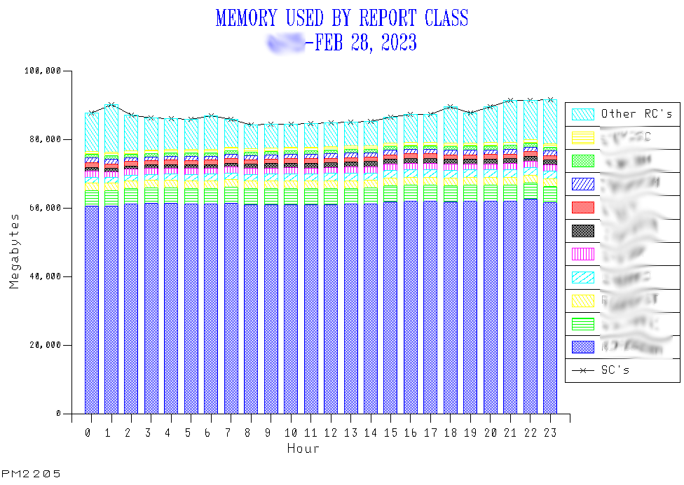
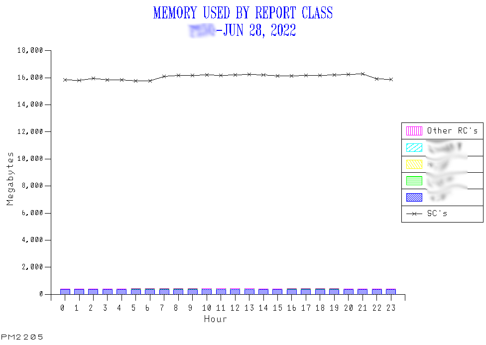
Here are a couple of examples – from different customers.

I’ve graphed two things on the one graph:

  1. The total service class view of memory – as a line.
  2. The report class view of memory – as a stack.

To make the graph readable I only plot the top 15 report classes individually. The remainder I roll up. I’d be surprised if there were much in the “other” category.

So let’s look at an example where there is good agreement between report class memory and service class. Here the service class line overlays the top of the stack.

And here’s an example where the report class coverage is very poor, relative to the service class view.

By the way, I’ve recently come across a customer with no report classes.

Granularity

Suppose you have good coverage by report classes. That can be achieved without yielding much benefit.

If you have very few report classes but between them they sum up to the service class view that doesn’t help much. Sometimes customers define report classes for aggregating service classes. I would hope any reporting tool could do the aggregation for you. I consider this to be a missed opportunity.

I’d rather see report classes used to break down service classes. I think this was the original WLM intention and this is perhaps why the limit is so high.

You could use report classes to keep track of memory used by a bunch of cloned CICS regions, for example. For this to be useful they wouldn’t be all the regions in a specific service class. I suppose you could track individual regions this way, too.

And you might well use report class SMF 72-3 for just such a purpose: The above (R723CPRS) formula is much more accurate than what SMF 30 currently has.

Another example might be to tally all the CPU used by jobs in a particular job class. This is especially useful where multiple job classes share the same service class – as is almost universal.

Equally, you might break out individual address spaces from SYSTEM. Particularly those, such as XCF, that start too early to yield SMF 30 intervals records.

One quite common case is aggregating address spaces for a Db2 subsystem. Here the IRLM address space ought to be in SYSSTC and the other “Db2 Engine” address spaces in a notional “STCHI” service class. You might well combine the two.

A Caution On Memory Reporting

There’s something else worth mentioning: The above are standard graphs we call “PM2205”, relying only on SMF 72-3. I didn’t show you one we call “PM2200”.

As I alluded to above, not all memory is captured for a report (or service) class. For example, common areas and memory for logically swapped address spaces. (The latter mostly affects TSO and Batch – and logically swapped address spaces consume memory but not service.)

So PM2200 has an additional job to do: Working to ensure all allocated memory is in the stack up; PM2205 doesn’t as it would get too busy if it also had eg CSA in. By the way, you get the common area storage from a combination of SMF 71 (Paging Activity) and 78-2 (Virtual Storage Activity) data.

In PM2200 we also subtract the total memory usage – from whatever source – from SMF 71’s total memory usage. Unimaginatively we call it “other” and usually it’s quite small.

One other thing PM2200 does – as it uses SMF 71 – is relate all the above to the amount of memory online to the LPAR. (No RMF data shows anything above activated LPARs., though it does speak to the freshly important Virtual Flash Memory (VFM).)

Conclusion

I would like installations to think about their use of report classes – to make sure they are truly useful. Many of the things you can do with SMF 30 you can do more readily with the right set of report classes. I am keen on customers learning how to get the full value out of SMF 30 but often SMF 72-3 does the job just as well, if not better.

So I’d be keen for customers to collect SMF 30 interval records – which most of them already do. You just don’t always have to process them to get what you want.

And, as this post majored on memory as an example of the value, I’d like us all to continue to evolve our reporting. PM2205 was certainly a recent evolution in our code.

And – the overall message of this post – do think carefully about your report class structure.

CF LPARs In The GCP Pool?

This post is about whether to run coupling facility (CF) LPARs using general purpose processors (GCPs).

It might be in the category of “you can but do you think you should?”

I’d like to tackle this from three angles:

  • Performance
  • Resilience
  • Economics

And the reason I’m writing about this now is the usual one: Recent customer experiences and questions.

Performance

What kind of performance do you need? This is a serious question; “Quam celerrime” is not necessarily the answer. 🙂

A recent customer engagement saw CF structure service times of around 1500μs. This is alarming because I’m used to seeing them in the range 3-100μs. This does, of course, depend on a number of factors. And this was observed from SMF 74 subtype 4 data.

You might be surprised to know I thought this was OK. The reason is that the request rate is extraordinarily low.

So what’s wrong with the inherent performance of CF LPARs in the GCP Pool? Nothing – so long as they are using dedicated engines, or at any rate not getting delayed while other LPARs are using the GCP engines.

But see Economics below.

So just like running on shared CF engines, really.

So the customer with the 1500Îźs service time was using a CF LPAR in the GCP pool capped with a very low weight. So, basically starved of CPU.

It turns out that the request rate being very low means the applications aren’t seeing delays and there is no discernible effect on the coupled z/OS systems. And that’s what really counts.

Resilience

By the way, the word is “resilience”. (Even the phone I’m writing this on says so.) I’m having to get used to people saying “resiliency” (which my phone is accepting of but not volunteering).

Having the CF LPARs in the same machine as the coupled z/OS LPAR has resilience considerations. Lose the machine and you have recovery issues.

Note the previous paragraph doesn’t mention processor pools. That was deliberate; it doesn’t matter which pool the CF LPAR processors are in, from the resilience point of view.

Economics

The significant question is one of economics: If you’re running on GCP pool engines these, of course, cost more than ICFs.

For modern pricing schemes I don’t think CF LPARs in the GCP pool cost anything in terms of IBM software. But there might well be software pricing schemes where they do.

And then there’s the question of maintenance.

All in all, the economics of placing a CF LPAR in the GCP pool will depend on spare capacity.

Conclusion

Yes you can, and just maybe you should. But only if the performance and economic characteristics are good enough. They might well be.

And you’ll see I’ve deliberately couched this in terms of “this is little different from any Shared CF engine situation”. The main difference being the economics.

One final point: if you need to have a CF LPAR and you’re on sufficiently old hardware you might have little choice but to squeeze it into a GCP pool. But do it with your eyes open. Unless you’d like to consider the benefits of a z16 A02 or z15 T02 – eg for production Sysplex designs .

Like You Know?

Three recent events led to this blog post:

  • I was driving a while back and listening to podcasts. Two in particular by highly experienced podcasters who are very articulate.

  • Meanwhile I’d just completed editing a podcast episode of my own. (This was Episode 32, which you might have listened to already.)

  • And a few weeks before that I was involved in a debate on an online forum about editing podcasts.

The common thread is humanity in the finished product. Versus professionalism, I suppose.

The online debate saw me advocating leaving some “humanity” in recordings, whereas others wanted “clean” recordings.

The podcasts I listened to today had “um”, “er”, “you know”, “like” aplenty. Because of editing and the debate online I was listening out for this. These “verbal tics” did not detract at all. Indeed the speakers sounded informal and human.

Now, it has to be said I’ve met all these podcasters – and would expect to be able to have good, friendly conversations when we meet again.

To bring this to Marna’s and my podcast, we are striking a particular pose. A genuine one but a conscious one: While we both work for IBM neither of us is making formal statements on IBM’s behalf. And, while we might have the tacit encouragement of our management, we’re not directed by them. In short, we don’t consider our podcast a formal production but just two friends having fun making a contribution.

If we were scripted and professionally produced we’d sound a lot different. And I think our episode structure would be different. And so would the content.

Having said that, I have two principal aims when editing:

  • Reduce the incidence of “um” etc to a listenable level.
  • Faithfully reproduce the conversation.

To that end, I generally don’t move stuff around or edit for content. I also try to do the easy edits and, beyond that, leave a few verbal tics in.

So you won’t get clean recordings from us. But you’ll get what we’re thinking, with some humanity left in.

And I’d say this song wouldn’t work without “you know”. 🙂

Mainframe Performance Topics Podcast Episode 32 “Scott Free”

Episode 32 was, as always a slow train coming. I think it’s a fun one – as well as being informative.

It was really good to have Scott back, and we recorded in the Poughkeepsie studio, just after SHARE Atlanta, March 2023.

Talking of which, the aftershow relates to SHARE. It’s a classic example of “today’s crisis is tomorrow’s war story”.

Anyhow, we hope you enjoy the show. We enjoyed making it.

And you can get it from here.

Episode 32 “Scott Free” Long Show Notes

Our guest for two topics was Scott Ballentine of z/OS Development, a veritable “repeat offender”. Hence the “Scott Free” title.

What’s New

Preview of z/OS 3.1

Mainframe – SMFLIMxx Parmlib Member

We discussed SMFLIMxx with Scott.

SMFLIMxx is a parmlib member, as a IEFUSI exit replacement. Its function is related to storage and specifying limits. Functions are delivered as continuous delivery. Two examples are

  • The SAF check
  • Number of shared pages used

In z/OS 3.1 customers will be able to specify Dedicated Real Memory Pools to assign memory to a specific application, like zCX. You will be able to use all frame sizes – 4KB, 1MB, and 2GB.

Performance – Open Data Sets, Part 1

This, the first of two topics on open data sets, was also with Scott. He’s very much the Development expert on this.

The main use for having very many open data sets (think “100s of thousands”“) is for middleware, most notably Db2.

Most of the constraint relief in this area is moving control blocks above the 2GB bar. In ALLOCxx you have to code SWBSTORAGE with a value of ATB to put SWB (Scheduler Work Block) control blocks above the bar. Applications need to exploit the service – or it has no effect.

Monitoring virtual storage is key here, and remains important: Factors such as the number of volumes for a data set affects how much memory is needed, so virtual storage estimation is difficult to do.

You can probably guess what Part 2 will be about.

Topics – Evolution of a Graph

Martin explored the large improvements he’s made with his custom graphing programs. (He already posted about what he sees with one of them here.) But this topic wasn’t about the technical subject of the graph, more the evolution from something “meh” to something much better. The evolution process was:

  • Start with a query that naively graphs database table rows and columns, with labels generated by the database manager and fixed graph titles. Not very nice, not succinct, not very informative.
  • Generating the titles with REXX, giving them more flexibility and allowing additional information to be injected.
  • Using REXX to drive GDDM directly – which enabled a lot of things:
  • REXX was able to generate many more data points and to plot them directly. (In particular the code is able to show what happens at very low traffic rates whereas previously it had had to be restricted to the higher traffic rates.)
  • REXX could generate the series names, making them friendlier and more informative.

The purpose of including this item, apart from it being a fun one, is Martin encourages everybody to evolve their graphs, to tell the story better, to run more efficiently, and to deal with underlying technological change. Don’t put up with the graphing you’ve always had!

Customer Requirement

ZOSI-2195 “Extended GDG causes space issues”, has been satisfied: IGGCATxx’s GDGLIMITMAX with OA62222 on V2.3.

On The Blog

Marna’s NEW blog location is here. There are three new posts:

Martin has quite a few new blog posts here:

So It Goes.