The CPU That You Do

(Originally posted 2015-10-31.)

It’s difficult to write about a live situation for two reasons:

• You don’t want to spoil the surprise.
• You mustn’t expose the customer.

Actually, make that three reasons:

• You don’t know how it’s actually going to turn out. 🙂

So why am I writing at all?

Well, the big engagement my team are involved in exemplifies the method for tuning CPU down, with a twist or two of its own. It’s the outline of that method I want to share with you.

At its simplest it’s very simple indeed:

Take The Large CPU Numbers And Make Them Smaller

But in this case (as in so many others) it’s not quite so simple. There are two complicating factors, one of which is universal, the other only sometimes present.

1. Which metric of CPU matters?
2. How do you handle multiple machines with, usually, diverse processor configurations?

The Relevant CPU Metric

For most customers the relevant metric is Peak Rolling 4-Hour Average. In our case it happens to be total CPU seconds.[1]

For the Peak Rolling 4-Hour Average (R4HA) one of the options is to depress the peaks, perhaps by displacing work in time.[2]

As an example consider the following (typical) pattern:

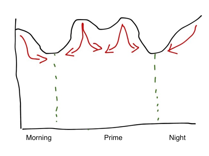
It has overnight batch intensiveness and two day time peaks. The red arrows show how you might try to displace work – as well as actually reducing the CPU consumed.

If you’re paying based on CPU seconds the area under the curve is what matters and the displacement option isn’t a good one. So you have to rely on reducing CPU seconds by tuning.

Actually, you could reduce the CPU load by shooing work away.[3] But I don’t think you generally want to.

Multiple Machines

Multiple machines pose a problem in that they often have diverse configurations and engine speeds. For the purposes of this exercise I’ve examined the Service Units Per Second and used the ratio across the LPARs to derive the relative engine speed.

The emphasis is deliberate in the previous sentence because, when you read on, the inaccuracy this introduces is irrelevant to the exercise: Deciding where to expend effort doesn’t need much accuracy.

It turns out the SU/Sec numbers varied by up to 10% across the whole estate – so I treated them all as the same. For this study it’s a nice simplification and I’m confident we have found the big handfuls of CPU.

Take The Big Numbers And Make Them Smaller

This is, of course, a recursive process – and it’s classic problem decomposition. This diagram summarises it.

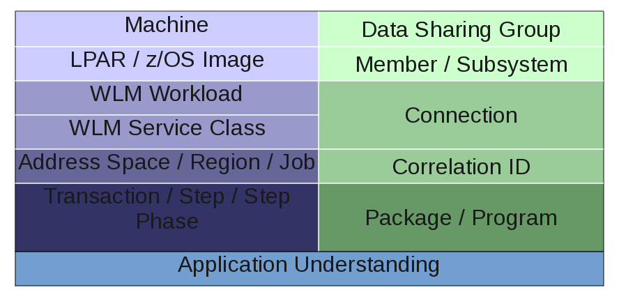
I’ve divided the diagram into two hierarchies [4] that more or less meet towards the bottom:

• On the right side we have DB2.
• On the left side we have “System” and similar stuff.

By side I don’t mean to imply that in a competitive sense, just literally sides of the diagram and as a label to aid division of labour.

System Side

The sequence of Machine then LPAR then Workload then Service Class then Address Space then… is entirely obvious and sensible. And you’d use such data as:

• SMF 70 – for the top layers.
• SMF 72 – for Workload and Service Class (Period) (and Report Class).
• SMF 30 – for address spaces, jobs and steps.

DB2 Side

In fact this side is generally handled by my DB2 colleague but, having done this in the past, I know:

• Data Sharing Group / Member / Subsystem start with Statistics Trace.
• The rest use Accounting Trace.

Actually, in this study I did look at DB2 Accounting Trace for two specific purposes:

• For DDF to get detailed information on which external applications were driving mainframe CPU when accessing DB2.
• For Batch to understand a little more about job steps’ use of CPU, for example whether Class 1 (“total”) or Class 2 (“in DB2”).

But my DB2 colleague looked at the myriad ways the subsystems could be tuned to reduce CPU. He raised an interesting point: If the DB2 subsystem is tuned wholesale doesn’t that mean the System-side CPU picture will change? Yes it does, but I think the balance of risk that large chunks of CPU will suddenly become unworthy of tuning because of DB2 subsystem tuning is small. (So work should proceed in parallel on both sides of the diagram.)

Application Understanding

This is where the magic happens:

By bringing together the System-side and DB2-side decompositions you should have quite a precise view of the moving parts that need tuning.

It’s time to wield the scalpel, now the body scanner has told you where to make the cuts.

---

So the above is sketchy, right? But it is a methodology as it’s systematic and yes I do have tools to implement it.

Do I have all the tools I could want? [5] Actually the sheer scale of this engagement has led me to believe one could build better tools – based off our current tools – that could make this go much quicker. Getting to build them any time soon is a matter of priorities.