Engineering – Part Four – Activating And Deactivating LPARs Causes HiperDispatch Adjustments

(This post follows on from Engineering – Part Two – Non-Integer Weights Are A Thing, rather than Engineering – Part Three – Whack A zIIP).

I was wondering why my HiperDispatch calculations weren’t working. As usual, I started with the assumption my code was broken. My code consists of two main parts:

• Code to build a database from the raw SMF.
• Code to report against that database.

(When I say “my code” I usually say “I stand on the shoulders of giants” but after all these years I should probably take responsibility for it.) 🙂

Given that split the process of debugging is the following:

1. Check the reporting code is doing the right thing with what it finds in the database.
2. Check the database accurately captures what was in the SMF records.

Only when those two checks have passed should I suspect the data.

Building the database itself consists of two sub stages:

1. Building log tables from the raw records.
2. Summarising those log tables into summary tables. For example, averaging over an hour.

If there is an error in database build it is often incorrect summarisation.

In this case the database accurately reports what’s in the SMF data. So it’s the reality that’s wrong. 🙂

A Very Brief Summary Of HiperDispatch

Actually this is a small subset of what HiperDispatch is doing, sufficient for the point of this post.

With HiperDispatch the PR/SM weights for an LPAR are distributed unevenly (and I’m going to simplify to a single pool):

1. If the LPAR’s overall weight allows it, some number of logical processors receive “full engine” weights. These are called Vertical Highs (or VH’s for short). For small LPARs there could well be none of these.
2. The remainder of the LPAR’s weight is distributed over one or two Vertical Mediums (or VM’s for short).
3. Any remaining online logical processors receive no weight and are called Vertical Lows (or VL’s for short).

Enigma And Variations

It’s easy to calculate what a full engine’s weight for a pool is: Divide the sum of the LPARs’ weights for the pool by the number of shared physical processors. You would expect a VH logical processor to have precisely this weight.

But what could cause the result if this calculation to vary. Here the maths is simple but the real world behaviours are interesting:

• The number of physical processors could vary. For example, On-Off Capacity On Demand could add processors and later take them away.
• The total of the weights for the LPARs in the pool could vary.

The latter is what happened in this case: the customer deactivated two LPARs on a machine – to free up capacity for other LPARs to handle a workload surge. Later on they re-enabled the LPARs, IPLing them. I’m not 100% certain but it seems pretty clear to me that IPLing doesn’t cause the LPAR’s weights to come out of the equation; I’m pretty sure IPLing doesn’t affect the weights.

These were two very small LPARs with 2–3% of the overall pool’s weights each. But they caused the above calculation to yield varying results:

• The “full engine” weight varied – decreasing when the LPARs were down and increasing when they were up.
• There was some movement of logical processors between VH and VM categories.

The effects were small. Sometimes a larger effect is easier to debug than a smaller one. For one, it’s less likely to be a subtle rounding or accuracy error.

The conversion of VH’s to VM’s (and back) has a “real world” effect: A VH logical processor is always dispatched on the same physical processor. the same is not so true for a VM. While there is a strong preference for redispatch on the same physical, it’s not guaranteed. And this matters because the cache effectiveness is reduced when a logical processor moves to a different physical processor.

So, one recommendation ought to be: If you are going to deactivate an LPAR recalculate the weights for the remaining ones. Likewise, when activating, recalculate the weights. In reality this is more a “playbook” thing where activation and deactivation is automated, with weight adjustments built in to the automation. Having said that, this is a “counsel of perfection” as not all scenarios can be predicted in advance.

What I Learnt And What I Need To Do

As for my code, it contains a mixture of static reports and dynamic ones. The latter are essentially graphs or the makings of – such as CSV files.

Assuming I’ve done my job right – and I do take great care over this – the dynamic reports can handle changes through time. So no problem there.

What’s more difficult is the static reporting. So, one of my key reports is a shift-level view of the LPAR layout of a machine. In the example I’ve given, it had a hard time getting it right. For example, the weights for individual LPARs’ VH processors go wrong. (The weight of a full processor worked in this case – but only because the total pool weight and number of physical engines didn’t change. Which isn’t always the case.)

To improve the static reporting I could report ranges of values – but that gets hard to consume and, besides, just tells you things vary but not when and how. The answer lies somewhere in the region of knowing when the static report is wrong and then turning to a dynamic view.

In particular, I need to augment my pool-level time-of-day graphs with a stack of the LPARs’ weights. This would help in at least two ways:

• It would show when weights were adjusted – perhaps shifting from one LPAR to another.
• It would show when LPARs were activated and de-activated.

A design consideration is whether the weights should stack up to 100%. I’ve come to the conclusion they shouldn’t – so I can see when the overall pool’s weight changes. That reveals more structure – and I’m all for not throwing away structure.

Here’s what such a graph might look like:

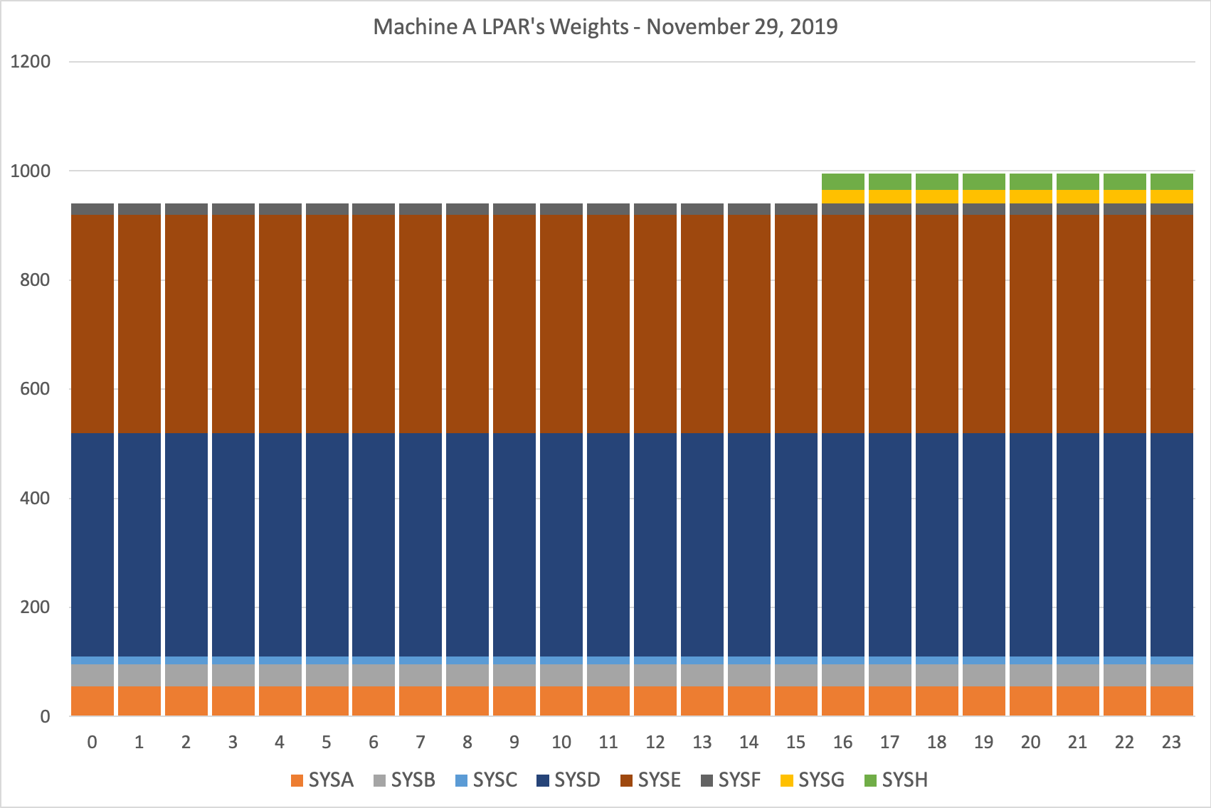
In this spreadsheet-driven mockup I’ve ensured the “now you see them now you don’t” LPARs are at the top of the stack.

I don’t know when I will get to this in Production code. As now is a particularly busy time with customer studies I probably should add it to my to-do list. But I’ll probably do it now anyway… 🙂

Head Scratching Time

In this set of data there was another phenomenon that confused me.

One LPAR had twelve GCPs online. In some intervals something slightly odd was happening. Here’s an example, from a single interval:

• Logical Processors 0–4 had polar weights (from SMF70POW as calculated in Engineering – Part Two – Non-Integer Weights Are A Thing) of 68.9. (In fact there was a very slight variation between them.)
• Logical Processor 5 had a polar weight of 52.9.
• Logical Processor 6 had a polar weight of 12.6.
• Logical Processors 7 to 11 had polar weights of 0.

If you tot up the polar weights you get 410 – which checks out as it’s the LPAR’s weight in the GCP pool (obtained from other fields in the SMF 70 record).

Obviously Logical Processors 0, 1, 2, 3, and 4 are Vertical High (VH) processors – and bits 0,1 of SMF70POF are indeed “11”.

But that leaves two logical processors – 5 and 6 with non-zero, non-VH weights. But they don’t have the same weight. This is not supposed to be the case.

Examining their SMF70POF fields I see:

• Logical Processor 5 has bits 0,1 set to “10” – which means Vertical Medium (VM).
• Logical Processor 6 has bits 0,1 set to “01” – which means Vertical Low (VL).

But if Logical Processor 6 is a VL it should have no vertical weight at all.

Well, there is another bit in SMF70POF – Bit 2. The description for that is “Polarization indication changed during interval”. (I would’ve stuck a “the” in there but nevermind.)

This bit was set on for LP 6. So the LP became a Vertical Low at some point in the interval, having been something else (indeterminable) at some other point(s). I would surmise VL was its state at the end of the interval.

So, how does this explain it having a small but non-zero weight? It turns out SMF70POW is an accumulation of sampled polar weight values, which is why (as I explained in Part Two) you divide by the number of samples (SMF70DSA) to get the average polar weight. So, some of the interval it was a VM, accumulating. And some of the interval it was a VL, not accumulating.

Mystery solved. And Bit 2 of SMF70POF is something I’ll pay more attention to in the future. (Bits 0 and 1 already feature heavily in our analysis.)

This shifting between a VM and a VL could well be caused by the total pool weight changing – as described near the beginning of this post.

Conclusion

The moral of the tale is that if something looks strange in your reporting you might – if you dig deep enough – see some finer structure (than if you just ignore it or rely on someone else to sort it out).

The other, more technical point, is that if almost anything changes in PR/SM terms – it can affect how HiperDispatch behaves and that could cause RMF SMF 70–1 data to behave oddly.

The words “rely on someone else to sort it out” don’t really work for me: The code’s mine now, I am my own escalation route, and the giants whose shoulders I stand on are long since retired. And, above all, this is still fun.