Drawers And More

Late last year I wrote a blog post: Drawers, Of Course. I’ll admit I’d half forgotten about it. Now that a few months have passed it’s time to write about at least part of it again.

So why write about it again now?

1. I’ve so much more experience with the instrumentation I described in that post.
2. My tooling has come on in leaps and bounds.

You’d think the two were related, and I suppose they are. But these two points give me the structure for this post.

Experience

Here I’m primarily concerned with learning how the data behaves – and what it shows us about machines’ behaviour.

My customer set has expanded, of course. Notable new data points are single drawer machines (Max39 for z16) and the other kind of four drawer machine (Max168). Both of these lead to different thoughts:

• One of the single drawer machines really should become a two-drawer machine when it’s upgraded from z15 to z16. Actually the one huge LPAR should be split before that happens.
• The Max168 obviously has a lower maximum number of characterisable engines in a drawer, compared to the Max200.

Some of the experience gain, though, is best left to when I talk aboutTooling. I’ve evolved my thinking about storytelling in this area – basically by doing it the hard way i.e. without adequate tools.

Sometimes, though, seeing whether a line of discussion even works in customer engagements is valuable. This time is no exception; This is indeed of value to customers. Even if, as in one case, I told a customer “all your LPARs fit very nicely in one drawer; Indeed most fit in one Dual Chip Module (DCM)”.

And some situations have seen me say “fine with the workload at the level it is but growth could easily take you beyond a drawer so don’t assume future processors will bail you out”.

Tooling

One of the reasons I didn’t show pictures in Drawers, Of Course is I wasn’t happy with the tooling I had. To be fair it was a first go with the new instrumentation so it was

• Cumbersome to operate
• Unable to tell a consumable story

In the intervening months I’ve made progress on both of those. So now is the time to share some of the fruits of that development work.

What I had then is some REXX for reading in SMF 70-1 records and writing one line per Logical Processor Data Section – as a CSV. I did at least have a sortable timestamp.

This produces a big file that requires you to cut and paste a given LPAR’s logical processors for a specific RMF interval into another CSV file – for a point-in-time view. And that cutting and pasting required a manual search for the lines you want. And a longitudinal view of a core was a pain to generate.

It also didn’t show offline processors. So, from interval to interval, a logical processor might come and go in its entirety. Not good for graphing. And not good for spotting it going on and offline.

So I wrote a shell script (“filterLogicals”) to process the big CSV file. It uses egrep to do one of two things:

1. Extract the lines for a given LPAR (or “PHYSICAL”) for a specified RMF interval.
2. Extract the lines for a given logical engine (for a single LPAR) for all intervals.

These two capabilities unlock some possibilities.

Having got the lines for a given LPAR (or PHYSICAL) there remains the problem of graphing or diagramming.

My current opinion is that you don’t really care which logical processor has its home address on which drawer / Dual Chip Module / chip. Mostly you care about how many of each type and polarity have their home addresses on each drawer / DCM / chip. My experience is that level of summary tells a nice story really quite well.

So I wrote a piece of python (“logicals” – which I shall probably rename) which takes the single interval output and summarises it as a CSV ready for Excel to turn into a graph. It can tell the difference between two cases:

1. Physical processors (from “PHYSICAL”).
2. Logical processors – for any other LPAR.

I’m still convinced that the so-called home addresses for “PHYSICAL” are actually where the physical cores are. Here’s an example

You can see

• The GCPs and zIIPs are in Drawers 1 and 2.
• The ICFs are in Drawer 4. (If there were IFLs I’d expect them to be in the higher drawers, too.)
• Drawer 1 has 39 characterised cores (which is the limit on this machine).
• Drawer 2 has 36 characterised cores.
• Drawer 3 has 10 – and that is where one of the LPARs sits.
• Drawer 4 has 16.

I separate the DCMs by a single line and the drawers by three lines in the CSV.

I don’t attempt at this stage to combine all the LPARs for a machine. One day I might; I’d like to.

A design decision I made was to colour the GCPs blue and the zIIPs green. Vertical Highs (VHs) are dark, Vertical Mediums (VMs) medium 😃, Vertical Lows (VLs) light. Offline processors are not filled but the bounding box is the right colour.

Fiddling with colours like that is a pain in the neck. After quite a lot of effort I got AppleScript working to find the series and colour them appropriately. The result is this:

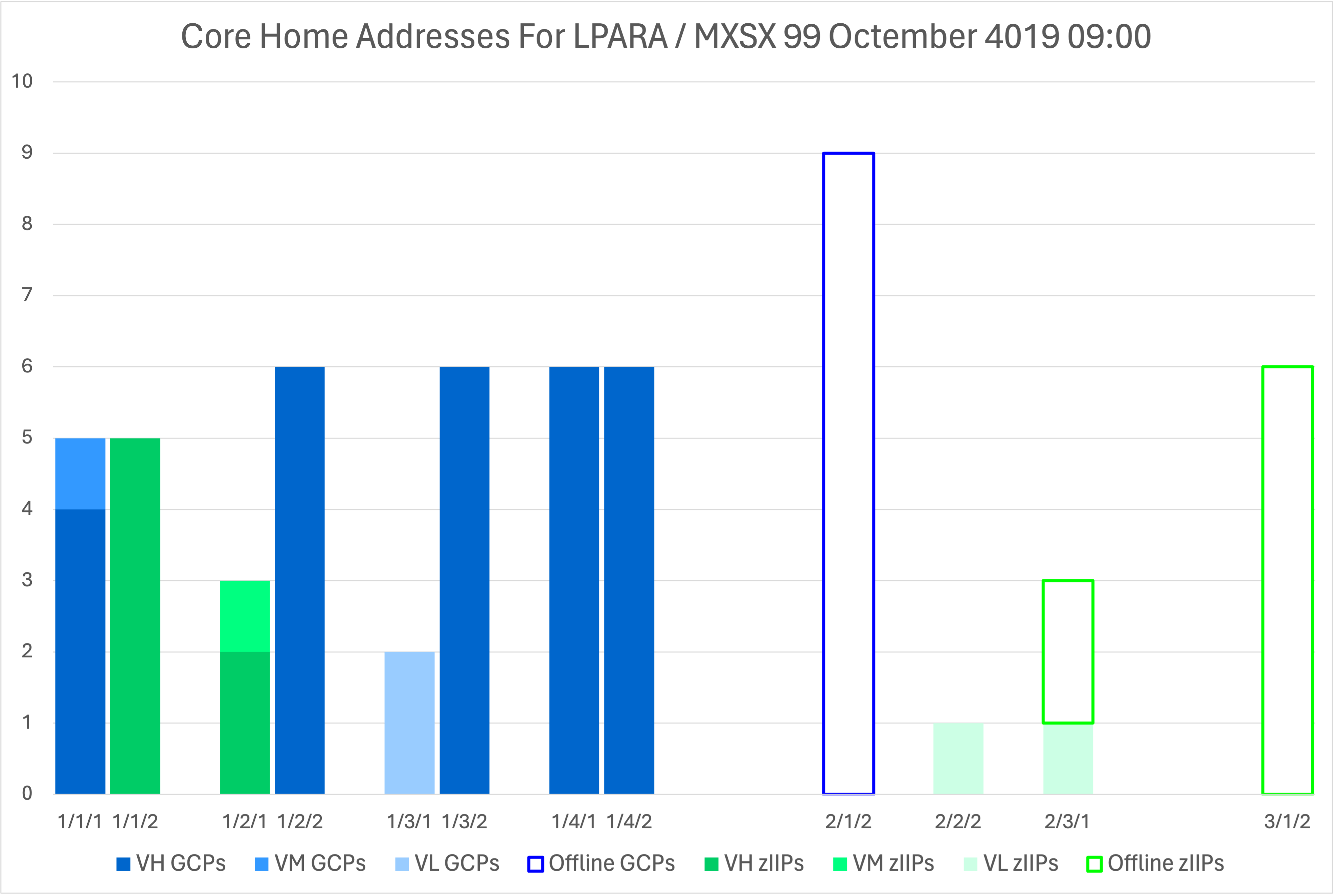
This is a real customer LPAR – from the same machine as the previous diagram. Notice how the offlines have home addresses. I will tell you, from experience, that when those processors are online they are likely to have different home addresses. It’s also interesting that there are 9 offlines on one chip – when there are only 8 cores on the chip; They can’t all be there when they come online.

The result of my effort is four pieces of code that make it very easy to see the home addresses for any LPAR at any instant in time. But I’ll keep fiddling with them. 😃

My REXX code now produces columns with Parked Time – for however many threads there are. But this can only be done for the record-cutting LPAR. Which reinforces the view you should cut SMF 70-1 records for all z/OS LPARs on a machine. HiperDispatch Parking is a z/OS thing, whereas HiperDispatch Polarity is a PR/SM thing.

One day I’ll be able to colour VL’s according to whether they are parked or not – or rather fractions of the interval they’re parked. That’s a not very difficult fix for the python code. That will show me, for instance, that those two VL’s off in another drawer are actually 100% parked (which they in fact are) – wherever in the machine they are dispatched.

Conclusion

There are a number of us looking at the new SMF 70-1 instrumentation. We tend to look at it in different ways, with different ways of diagramming and graphing.

I’ve described my tooling in a bit of detail because it’s actually in the kind of shape I could ship as part of a new open source project. No promises that I’d ever be allowed to do that but I’d be interested to know if this is something that people would find useful.

I should also mention that SMF 113 is a very good companion to SMF 70-1. Again, keep it on for all z/OS LPARs.

I’ve also laid a trap for myself; I wonder if you can spot my “hostage to fortune”. 😀

Making Of

I started writing Drawers, Of Course on a plane to Istanbul. Here I am again, doing exactly the same thing. And I know jolly well the topic of drawers will come up with this other customer’s workshop. It rarely doesn’t these days.

And I think so much of the topic of drawers that “Drawers, Of Course” has grown into a presentation I’ll be giving at GSE UK Virtual Conference, 23-25 April. By the way, we have an exciting stream of presentations on the z Performance & Capacity stream there.

One other point: You might ask “why so many bites at / of the cherry?” It’s my privilege in this blog to write about stuff as I learn. It might be embarrassing if something I write later on contradicted something I earlier said. But that’s a rarity and not that embarrassing. The point is as I learn (through book or experience) I share. Maybe one day I will consolidate it all into an actual book. I just don’t have the time or structure yet. And that might not be the right medium.

If you’ve made it this far you might appreciate that “Drawers, Of Course” could have been better as “Drawers, Of Cores”. 😀 Oh well.