(Originally posted 2008-07-29.)

Yesterday DFSORT announced a new set of functions – as PTF UK90013. The documentation for it can be found here.

Every year or so there’s a new set of DFSORT functions – and generally they’re “out of cycle” with z/OS releases – although they are incorporated into subsequent releases of z/OS. This means that fewer of you will know about the functions, particularly as we don’t make a big fuss about it at z/OS release announcement time. So you quite possibly, when you move to a new release of z/OS, get new DFSORT functions you don’t know about.

I’m privileged to call the DFSORT developers friends. And I get to “beta” the new code ahead of release. This time, due to other commitments (like the “Parallel Sysplex Performance Topics” Redbook), it’s been difficult to find the time to play much with the code.

So, what’s new?

Here are a few highlights:

• FINDREP makes it MUCH easier to do “find and replace” operations. Hence, presumably, the name. 🙂

  There are a number of ways of specifying the search string and its replacement. For example, you can specify multiple input strings that get changed to the same output string. You can also define pairs of strings so that you can find and replace multiple strings in one pass over the data. But you can also just specify a single string and its replacement.

  These strings can be specified as character strings (e.g C’XYZ’) or hexadecimal strings (e.g. X’FFAB’). Or as multiples (e.g 4X’FF’). And DFSORT Symbols can be used for C’XYZ’ and X’FFAB’ styles (but not the “multiplier” styles).

  You can specify search “margins”. So, you could specify that strings are to be sought between positions 11 and 71, for example.

  You can specify the maximum number of times find and replace is performed for a record. So you could specify for example only the first match is to be replaced.

  You can say what is to happen if a replacement operation causes the output record to become wider than the LRECL.

  If you don’t want the remainder of the record to be shifted left or right after a match you can specify that as well.

  All in all a nicely thought out set of options.

  Here’s an example I actually need today:

  OPTION COPY                             
  INREC FINDREP=(IN=(C'#@$'),OUT=(C'SYS'))
  

  All our systems have SMFIDs beginning “#@$” and our tooling currently has a problem with a “$” character in certain places. Replacing “#@$” with “SYS” gets us out of a hole. And it’s pretty much guaranteed that anywhere in the SMF records we see “#@$” is part of a SMFID. So preprocessing with FINDREP will help.

• Group operations (using WHEN=GROUP) allow you to identify and operate on groups of records.

  A group of records can be identified in one of two ways:

  • Every n records is a new group. (This uses the “RECORDS=” syntax variant.)
  • All the records between a header record and a trailer record is a new group. (This uses the “BEGIN=” and/or “END=” syntax variants.)

  Here’s an example, straight from the new documentation:

  INREC IFTHEN=(WHEN=GROUP,RECORDS=3,PUSH=(15:ID=3,19:SEQ=5)
  

  specifies groups of three consecutive records. Position 15 for 3 is an identifier that increments for each group. Position 19 for 5 is a sequence number that increments by 1 and restarts at the beginning of each group.

  In the above it’s the PUSH that actually edits the records.

  One thing to note: It’s entirely possible (but not in this example) that records fail to fall into any group. With BEGIN and END it’s possible to have records before the first BEGIN hit and after the last END hit and between an END hit and the next BEGIN hit. Here’s a way of detecting them:

  OPTION COPY
  INREC IFTHEN=(WHEN=GROUP,BEGIN=(1,5,CH,EQ,C'START'),END=(1,4,CH,EQ,C'STOP'),PUSH=(10:ID=1))
  OUTFIL FNAMES=REJECTED,INCLUDE=(10,1,CH,EQ,C' ')
  

  In the above case groups start with a record with “START” in them and end with records with “END” in them. The “PUSH” sets a flag for records in a group. The OUTFIL writes records to a sidefile where the flag wasn’t set.

  Just for grins, I tried a “mis-nesting” or “mis-bracketing” where the input stream was:

  START
  START
  STOP
  STOP
  

  The output was:

  START    
  1START    
  2STOP     
  2STOP
  

  So each “START” record starts a new group, regardless of whether the previous group was terminated with an “STOP” record. So the second “STOP” record isn’t part of any group. Still, I expect most applications will have “well formed” input data, cough cough. 🙂

  RECORDS, if specified with BEGIN or END has a slightly different role to when it appears on its own. It limits the number of records in a group.

One of the nice things about the above is you can fit them into an IFTHEN “pipeline”. IFTHEN lets you pass records through a sequence of filters – much like real pipelines. WHEN=GROUP, in particular is always used within IFTHEN, even if there are no other filters (or “stages” as they’re sometimes known). Also, WHEN=GROUP can be intermixed with WHEN=INIT but must before the other WHEN clause types.

The other significant enhancements are all related to ICETOOL:

• DATASORT is a new operator that allows you to sort the data records in a data set without sorting the header or trailer records. Header and trailer records are copied in their original order, continuing to bracket the sorted data records.

  You use HEADER, FIRST, HEADER(n), FIRST(n) to denote the first one or n records are the header. Similarly, TRAILER, LAST, TRAILER(m), LAST(m) denote the last one or m records are the trailer.

  You can use OUTFIL to post-process the entire output stream, including header and trailer records.

• SUBSET is a new operator that selects records based on their record number, for example the first 5 records – FIRST(5). You can specify whether subsetting is done on the way into a sort or on the way out. Again you can use OUTFIL to post-process the records.

  NOTE: If you specify eg LAST(n) ICETOOL may have to call DFSORT twice. The first pass is to count the input records. The second is to actually write out to the output data set. Because the first pass doesn’t actually OPEN the output data sets this kind of two-pass approach is fine with a BatchPipes/MVS pipe as the output data set.

• The SELECT operator is enhanced to allow you to select the first n records with each key or the first n duplicate records with each key. This is useful for a “top list” approach. (I once did something similar with REXX driving DFSORT.)

  While there are FIRST(n) and FIRSTDUP(n) forms there aren’t LAST(n) and LASTDUP(n) forms. But Example 1 in the documentation shows how you get round that using a different sort sequence.

• The SPLICE operator is enhanced with a new keyword: WITHANY. (As if having WITHEACH and WITHALL wasn’t confusing enough already.) 🙂

  WITHANY creates one output record for each set of duplicates. The first duplicate is written out with with the non-blank values of each subsequent duplicate spliced onto it for specified fields. (“Spliced onto” or “Spliced into”?) 🙂

  The documentation gives a far better description of this than I can here. Which is another way of saying “SPLICE confuses the heck out of me.” 🙂

• The DISPLAY operator now allows you to display counts in reports. Formerly you could display totals, maxima, minima and averages (and the “sub” variants of those).

• The DISPLAY and OCCUR operators have greatly enhanced title capabilities:

  • You can have up to 3 title lines.
  • Each can have up to 3 strings.

  This flexibility enables you to use DFSORT Symbols in titles, including System Symbols. To do the latter code something like:

  //SYMNAMES DD *System,S'&SYSNAME'Sysplex,S'&SYSPLEX'

  and then in ICETOOL control statements something like:

  TITLE('System: ',System)

• The COUNT operator has been enhanced to allow you to write its output to a data set. Previously it went to SYSOUT. So you could code something in the form:

  COUNT FROM(EMPIN) WRITE(EMPCT) - TEXT('Number of employees is ') - EDCOUNT(A1,U08) WIDTH(80)

  to get output like:

  Number of employees is 1,234,567

  A1 is a mask that puts commas in. U08 means “Use 8 digits”.

  COUNT also allows you to add to or subtract from the count with ADD(n) or SUB(m). If criteria like EMPTY are used it’s the modified record count that is used in the comparison (in this case to 0).

So there’s lots there to play with. And it’s available right now.

And if you want all the user guides for “recent” function PTFs go here.

(Originally posted 2008-07-11.)

A couple of days ago I attended the pilot of a “Web 2.0 and System z” workshop in the Boeblingen lab. I’m pleased to say the room was full – both with IBMers and non-IBMers. And I think my presentation – which was basically a rant about Web 2.0 Behaviours and why we should adopt them as mainframe folks 🙂 – went OK.

One of the things that was interesting about it was that on greeting Luis Suarez (@elsua on Twitter) we felt it natural to hug – though we’d never physically met before. I think that’s a testament to the power of relationships built through Social Networking. Oh, and I made new friends as a result of the workshop. So welcome @ansi, @frogpond and @rodet – all Twitter users.

Actually there were lots of things interesting about the workshop and another one will be running in the Autumn. I gather there’ll be some “hands on” then, which I’d encourage.

I’m wondering if other people would like to see such a workshop – in other parts of the world.

And it was nice to reprise my presentation the next day in front of WLM, RMF and Capacity Provisioning Manager (CPM) developers.

And now my copy of the O’Reilly book “Dojo: The Definitive Guide” has arrived. So I’m “Web 2.0’ed out” for the week. 🙂 Actually the book looks like it covers the ground quite well. I have a half-jesting rule of thumb: If there’s an O’Reilly book about a technology it’s probably ready. If there’s a “For Dummies” book on the subject it’s probably boring, dulle and passe. 🙂

(Originally posted 2008-07-11.)

In the same meeting with RMF Development as ERBSCAN / ERBSHOW was discussed we talked about Parallel Sysplex instrumentation. (Both XCF and Coupling Facility aspects.)

One thing I hadn’t noticed is the appearance of Subchannel Busy Percentage as a number in the following three places:

• In Monitor III
• In the Spreadsheet Reporter
• As Overview Condition (“SUBCHBP”)

I think you can do useful work with this but you have to know a few things about it:

• It is one system’s view.
• It is an estimate, derived from request rates and service times, both Sync and Async. Essentially you work out the request total time in the RMF interval and divide that by the interval length and the number of subchannels. The implicit assumption is that the service time is all subchannel busy time and that there is no other time when the subchannel is busy. It’s a moderately well-known formula, however.
• It says nothing about individual subchannel busy levels – nor about paths.

This topic is of interest to me for a couple of reasons:

• On our Residency in May / June we used coupling facilities that were attached by a mixture of ICB and ISC links. Two different link types between the same z/OS and the same coupling facility. It would’ve been really nice to see which link type actually got favoured.
• My suspicion is that customers would like to do more detailed connectivity analysis and tuning for their parallel sysplexes. For example, if a link doesn’t get used it’d be nice to know that and to be able to trouble-shoot it. (Perhaps someone left it connected as a 20km fibre suitcase.) 🙂

So, I’m wondering… Is link and connectivity information important? What do you need? And why? Or is the Subchannel Busy Percentage estimate good enough for you to work with?

Oh, and thanks to Matthias Gubitz for the phrase “Gutes tun und daruber sprechen” (“Do good and speak about it.”) 🙂 That’s probably the best reason for blogging and such like.

And the “neologism of the week” award goes to Harald Bender for the word “handisch”. Neither English nor German. 🙂 We believe he meant “by hand”. But for now I prefer “handisch”. 🙂

(Originally posted 2008-07-11.)

I mentioned ERBSCAN and ERBSHOW in this post from January. This is a handy pair of tools for displaying SMF records – most notably the ones produced by RMF. For the uninitiated you type ERBSCAN in ISPF 3.4 against an SMF data set and it pops up a list of SMF records. Typing ERBSHOW followed by the record number formats the record – especially well if it’s one that RMF produced.

And the prior post on ERBSCAN and ERBSHOW talked about the “x” parameter for ERBSHOW that enhances the formatting.

So, I was in Boeblingen for a different purpose this week and took almost 2 hours of the RMF Development team’s valuable time. 🙂 We talked about many things, including “futures”. There was, as usual, a good meeting of minds.

Matthias Gubitz mentioned an enhancement to ERBSCAN that is worth relating. It’s in z/OS Release 9, but it won’t’ve made the headlines…

The list of records that ERBSCAN produces is an ISPF Edit session. So you can do ISPF Edit things like using Find and Exclude All…

In the past I’ve used it to navigate to eg SMF 74-4 with “F ‘074.004’ and to find records cut by a specific SMF ID. So you can imagine what’s displayed affects usability…

Matthias added the following two items:

• For 72-3 (Workload Activity) the Service Class.
• For 74-4 (Coupling Facility Activity) the Coupling Facility name.

You can see that being able to search on these, perhaps going “Exclude All” first, is going to make finding the records you want – to ERBSHOW – much easier.

Well I think it’s going to save me time. 🙂

And the RMF guys mentioned to me that ERBSCAN / ERBSHOW seem to have become popular. I wonder why. 🙂

(Originally posted 2008-06-25.)

Many of you will have, by now, installed the Adobe AIR runtime. Most probably it will be to run something like Twhirl.

At this point many of you will be asking “what’s Twhirl?”

If I said it was a nice desktop application that makes using Twitter so much easier I hope you don’t ask “what’s Twitter?” 🙂

So, we’re beginning to see these desktop applications coded using Adobe AIR, which stands for “Adobe Integrated Runtime” (formerly “Apollo”).So, what’s special (if anything) about AIR?

In my experience, two things:

• AIR applications run across Mac, Windows (and in Alpha form) Linux.

  (In fact I installed the Linux AIR alpha plus Twhirl on my ASUS EEE PC some months ago. (Nice machine that EEE, by the way.) It worked fine within the limitations of the AIR alpha code.)

• It’s entirely possible to code up AIR applications using just a text editor. (in fact that’s precisely what I did.)

  My editor of choice, for whatever that’s worth, is Notepad++ on Windows. (And I’d rather not start an editor war here, thanks.) 🙂 And the EEE comes with the Kate editor, being built on Debian Linux.

  I like environments where there is little, if any, in the way of barriers to entry for programmers.

So what does an AIR application consist of?

In principle one can do fancy things with Adobe Flex Builder and .SWF files but that requires expensive tooling. But there is another way:

You can write an AIR application of arbitrary complexity with two files:

• A small XML file.

• Your HTML file which can also have javascript in, just like normal web pages. In fact your typical AIR HTML file could be thrown straight into a web browser and work just fine.(That is unless you use some of AIR’s special capabilities – which your javascript can detect the availability of and code around accordingly.) And I assume that when I say “your browser” I mean a standards-compliant one like Firefox. 🙂 Note: The flavour of AIR that uses HTML / Javascript is actually built around the Safari browser.

  So I really think the “this builds on what you already know” point makes it attractive to an awful lot of people.

This isn’t an AIR tutorial so I’m not going to give you samples of the small XML and html files. You can easily find those on the Web. I just want to leave you with the impression there isn’t much to it. And there is an O’Reilly pocket guide for AIR. (But there isn’t a “For Dummies” book for it – so that’s alright.) 🙂

There are alternatives – such as Mozilla’s XULRunner (whose user interface is based on XUL rather than HTML) and, I suppose, Microsoft’s Silverlight. But neither is as easy and “I just need a text editor and the SDK to do it” is pretty enticing.

So, I’m impressed at its simplicity, the fact it builds on HTML, XML and Javascript. And if you want to be able to build something that looks like a desktop application, complete with drag-and-drop and clipboard capabilities, this may well be a good fit for your needs.

I mentioned the SDK. It’s free (but it doesn’t run on Linux and I’ve not heard any suggestion that it will). It comprises two useful tools:

• ADL – which you use for testing
• ADT – which you use for packaging up your completed application. This involves signing the resulting .AIR file – and the ADT tool has the capability to enable you to be “self certifying” so that gets round the cost of getting a certificate from a more formal authority. But it does require users to trust you. 🙂

Both are simple to use.

So, I got a “Hello World” application up and running in about twenty minutes, and that even with typ(o)ing in the XML and HTML files from the O’Reilly book. Swiping from the Web would probably be quicker – but you’d learn less.

And now I’m proving remarkably productive at writing a full-scale application. What’s slowing me down – if anything – is my very basic CSS. And this application uses XMLHttpRequest and walks the DOM tree to build the window contents on the fly. All using standard javascript. Oh, and my CSS is rather more under control. 🙂 I just need to refactor it into multiple parts as all my CSS / HTML / Javascript is in the one file. Oh, and then there’s refactoring to use dojo. I’m told you can use dojo in an AIR application, so long as you ship the dojo runtime with it.

If you want to know more about AIR go to their blog. For Twhirl go here and, of course, Twitter is here.

Note: IBM doesn’t appear to have any commercial interest in AIR. And I certainly don’t. So I’m just telling you how I see it.

(Originally posted 2008-06-21.)

The same Kevin Keller I mentioned in this blog post is running a one day pilot of a “Web 2.0 and System z” workshop on July 8th, in IBM Böblingen. It’s designed for customers, though some of the audience will undoubtedly be IBMers. I’ve looked at the agenda and, while I’m on it, it’s a great agenda. 🙂 Actually it has the highly-acclaimed Luis Suarez on the agenda as well. (I’m looking forward to meeting Luis as, though we’ve talked many times using all the social media, we’ve never actually met before.)

If you want to attend the workshop – or would like more information – let me know and I’ll see what I can do. I don’t control the attendee list so I can’t promise you a place.

Though run by IBM Germany this workshop is in English.

I’m looking forward to this class tremendously: As my long-suffering audiences 🙂 know I’m keen that people and organisations realise there’s a lot of scope for doing Web 2.0 (or, more generally, modern) stuff on z/OS. So this workshop ought to be the proof of that.

(Originally posted 2008-06-20.)

Take a look at my German colleague Kevin Keller’s new blog in Web 2.0 and z/OS. I think you’ll be pleasantly surprised at what runs on z/OS that the rest of the world would regard as modern. 🙂

I say “modern” rather than “Web 2.0” because I feel the latter term is generally overused. What is really to the point is quite how much stuff could (and in many cases should) be implemented on z/OS, e.g. accessing DB2 (especially with the PureXML support in V9).

I’ve suggested to Kevin he might like to write additional posts on some of the products mention in his first mammoth post. I think some of them are going to prove remarkably easy to implement.

(Originally posted 2008-06-19.)

Hats off to Jonathan Feinberg (who’s created a number of neat sites inside IBM) for creating Wordle.

The above is a nice depiction of the keywords for my blog. Click on it for a bigger version.

Go to here to make your own from any sets of text you like.

(Originally posted 2008-06-16.)

I’m not sure if anyone’s done this before. Certainly I’ve not seen any results…

We’re beginning to write up some tests the “A Team” (Alain and Pierre) ran before their return to France. Which provides me with some test data. Fortunately I had a stab at mapping the new fields this data contains. One in particular is Stucture CPU (R744SETM)…

So, I got to plotting CPU per request against request rate (as well as elapsed time against request rate). I did this for two structures:

• LOCK1 – which has between 750 and 925 requests a second – based on 1 minute RMF intervals.
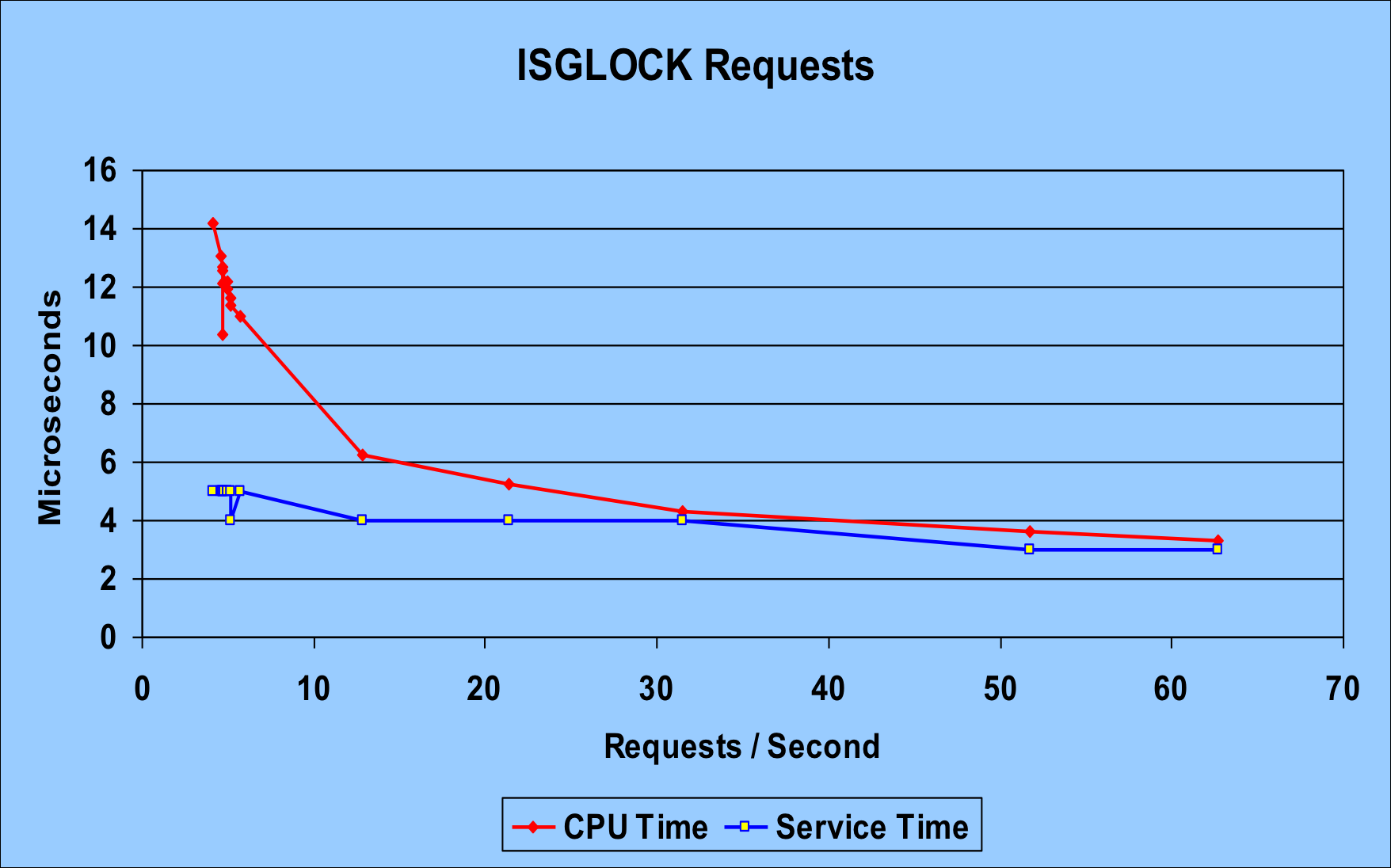
• ISGLOCK – which has between 5 and 65 requests a second.

The high request rate LOCK1 case is less interesting for the purposes of this discussion. The chart below is for ISGLOCK. I think it’s revealing.

The red line is the CPU time per request. Most importantly it goes down with the number of requests. That strongly suggests to me that there’s a “zero request rate” cost, which gets amortised over more requests as the rate increases. Now, some of this could just be Coupling Facility internal processes. Or it could be a cache effectiveness thing. And in any case maybe it’s RMF with its 1-minute intervals that’s driving the CPU consumption.

The blue line is the service time per request – which actually drops as the rate increases. This might be a “practice effect” or else some instrumentation effect. At any rate it drops rather less dramatically than the CPU time per request.

What’s also interesting is that the CPU time and the service time converge somewhat. You’d expect the service time to be more than the CPU time – for a request. But, as you can see from this blog entry that isn’t always the case.

So, the net result of this test is that there’s CPU to amortise over the requests and at lowish rates this can be enough to make it longer than the service time.

For ISGLOCK – locking with no record data payload – it’s pretty much all CPU time, so long as nothing else gets in the way. (Such as path / subchannel delays or extreme CPU queuing in the coupling facility. Or, more to the point, link latency.)

For LOCK1, the request rate was much too high to see the amortisation in action and CPU was always about 4μs vs service time of around 10μs per request. LOCK1 does have record data to manipulate.

There’s one other consideration, though: LOCK1 was in a coupling facility with a mixture of ISC and ICB links. ISGLOCK was in a coupling facility accessed using IC links. That probably accounts for some of the 10μs. for LOCK1 vs 3.5μs for ISGLOCK. In fact, the CPU time per request for LOCK1 was about 4μs out of the 10μs. Which suggests quite a bit of link latency.)

It’s a new-found frustration of mine that the instrumentation doesn’t tell me much about traffic by link or link type. (Earlier in the residency I messed around with channel activity and queuing record types. Perhaps I’ll have to mess with it again.)

In “real world” terms bear in mind, however, that the 50 requests per second and upwards cases are much more interesting and common. So typical behaviour is towards the right hand end of the graph and beyond.

(Originally posted 2008-06-12.)

It’s fair to say I’ve written very little in terms of book words these past two days. That’s because I’ve been “doing research” on how the cache structure counters really work. “Doing research” is a euphemism for “finding out how the heck the darned thing works”. Which is in itself a positive thing to do – but it does rather get in the way of writing stuff. 😦

There is a section in the SMF 74 Subtype 4 called the “Cache Data Section”. I thought you got one for each cache structure. It turns out you can get more than one. There are things inside cache structures called storage classes. So I trawled through all the customer data I have gathered over the past year and in only one> structure (not one customer) did I see a count of 2 sections. This for XBM. Even DB2, which uses multiple castout classes per structure, only has one storage class. So I don’t feel bad about my code assuming only one.

The other thing one needs to know – and it’s far more important – is that for every system connecting to a structure the Cache Data Section contains identical values. It’s rather like the Disk Cache statistics in SMF 74 Subtype 5: The controller / coupling facility maintains the stats. So it’s no use summing them.

When it comes to what’s in the section there are umpteen counters: 5 read counters, 5 write counters, 4 cross-invalidation counters and umpteen others. In my code we calculate read hit percentages, read-to-write ratios and lots of other things besides. Figuring out what all these counters mean and which ones are important is what’s euphemistically called “a work in progress”. 🙂

But the real learning point is that each exploiter does it differently. So, two examples:

• A store-through cache doesn’t do castouts. A store-in one does. And then there’s a “cross invalidation” cache that doesn’t either. But then it doesn’t actually store data to consider the fate of.
• DB2 Data Sharing with GBPCACHE(CHANGED) doesn’t write unchanged data to the cache structure.

And so it goes on.

I think it would be a noble aim to describe all these counters in terms that are related to exploiters. And also in terms we can all understand. Let’s hope it doesn’t remain just a noble aim. 🙂