In Automating Microsoft Excel I wrote about some basic manipulation of graphs in Excel for Mac OS, using AppleScript.
I’m writing about it again because of the paucity of examples on the web.
Here is an example that shows how to do a number of things in that vein.
tell application "Microsoft Excel"
    set c to active chart
    tell c

        set xAxis to (get axis c axis type category axis)
        tell xAxis
            set has title to true
        end tell
        set tx to axis title of xAxis
        set axis title text of tx to "Drawer / DCM / Chip"
        set font size of (font object of tx) to 14

        set yAxis to (get axis c axis type value axis)
        tell yAxis
            set has title to true
        end tell
        set ty to axis title of yAxis
        set axis title text of ty to "Core Count"
        set font size of (font object of ty) to 14

        set fore color of fill format of chart format of series "VH GCPs" to {0, 0, 255}


        set fore color of fill format of chart format of series "VM GCPs" to {51, 153, 255}

        set fore color of fill format of chart format of series "VL GCPs" to {185, 236, 255}
        set fore color of fill format of chart format of series "VL Unparked GCPs" to {185, 236, 255}
        set fore color of fill format of chart format of series "VL Parked GCPs" to {185, 236, 255}

        chart patterned series "VL Parked GCPs" pattern dark horizontal pattern

        tell series "Offline GCPs"
            set foreground scheme color of chart fill format object to 2
            set line style of its border to continuous
            set weight of its border to border weight medium
            set color of its border to {0, 0, 255}

        end tell

        set fore color of fill format of chart format of series "VH zIIPs" to {0, 255, 0}
        set fore color of fill format of chart format of series "VM zIIPs" to {96, 255, 180}
        set fore color of fill format of chart format of series "VL zIIPs" to {185, 255, 236}
        set fore color of fill format of chart format of series "VL Unparked zIIPs" to {185, 255, 236}
        set fore color of fill format of chart format of series "VL Parked zIIPs" to {185, 255, 236}

        chart patterned series "VL Parked zIIPs" pattern dark vertical pattern


        tell series "Offline zIIPs"
            set foreground scheme color of chart fill format object to 2
            set line style of its border to continuous
            set weight of its border to border weight medium
            set color of its border to {0, 255, 0}
        end tell

    end tell
end tell
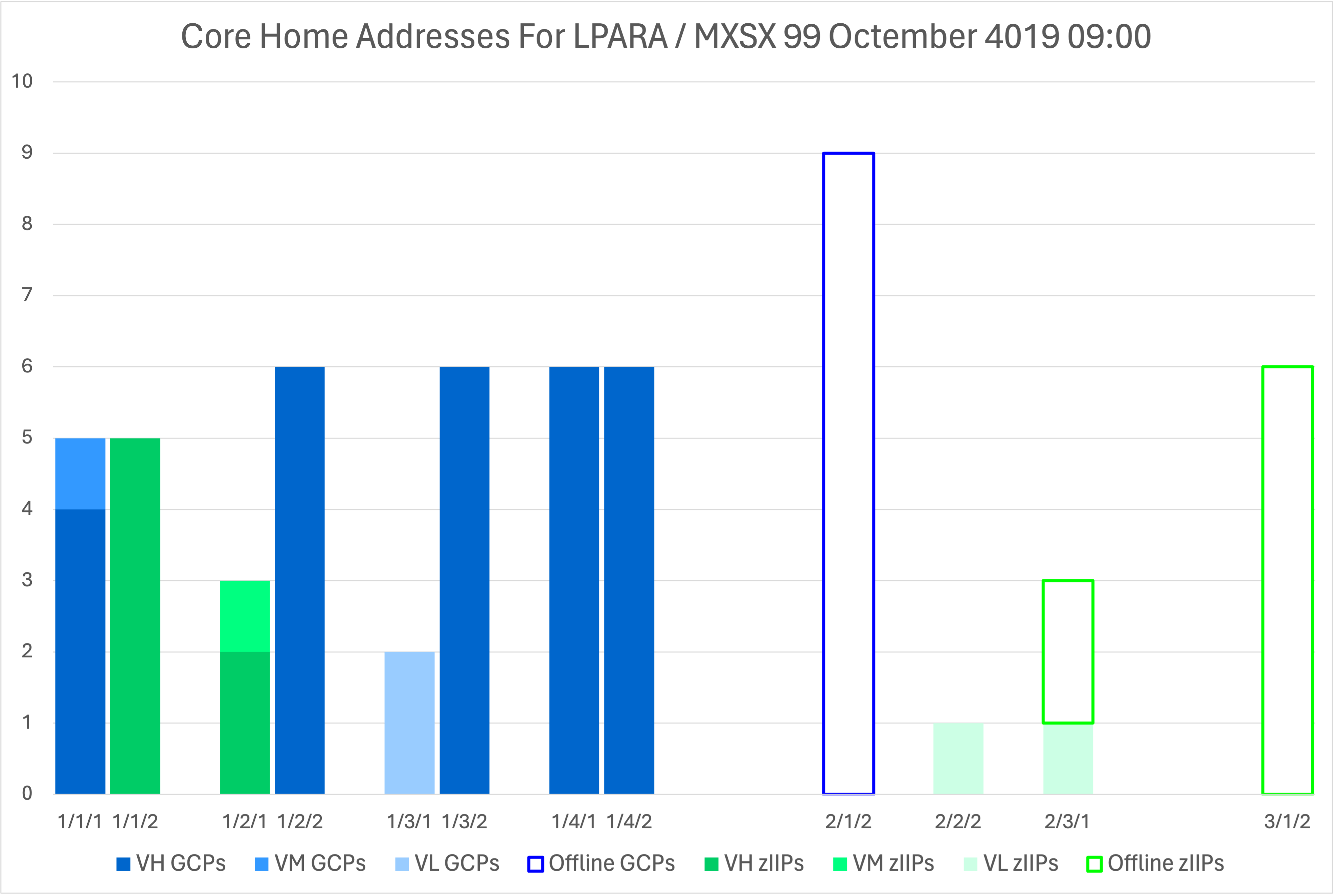
The above is the code I use to colour my drawer-level graphs.
Let me extract pieces that you might to use. (My assumption is that anybody reading this far got here because they came for AppleScript / Excel tips.)
Addressing The Active Chart
Everything in this post assumes you have selected a chart (graph) and want to manipulate it. The other snippets will need to be wrapped in this.
tell application "Microsoft Excel"
    set c to active chart
    tell c
        ...
    end tell
end tell
The point is to tell the active chart object what to do.
Manipulating Chart Axis Titles
First let’s manipulate the title of the x axis. Excel calls this the category axis.
The following
- Sets
xAxisto the category axis of our chart. - Turns on the title for the axis.
- Sets
txto the axis title object. - Sets its text to “Drawer / DCM / Chip”
- Sets its font size to 14 points
set xAxis to (get axis c axis type category axis)
tell xAxis
    set has title to true
end tell
set tx to axis title of xAxis
set axis title text of tx to "Drawer / DCM / Chip"
set font size of (font object of tx) to 14
Now the y axis title:
set yAxis to (get axis c axis type value axis)
tell yAxis
    set has title to true
end tell
set ty to axis title of yAxis
set axis title text of ty to "Core Count"
set font size of (font object of ty) to 14
The only real difference is we’re setting yAxis to what Excel calls the value axis.
Setting The Foreground Fill Colour For A Series
This one turned out to be quite difficult to figure out.
- You address a series in a chart by its legend value:
series "VH GCPs. - You get the chart format of the series:
chart format. - You get its fill format:
fill format. - You set its foreground colour (
for color a) using RGB (Red/Green/Blue) values. In this case full-on blue:`
The brackets in that last denote a list of values.
Put it all together and you get this:
set fore color of fill format of chart format of series "VH GCPs" to {0, 0, 255}
The main snippet has several of these.
Setting A Series Pattern
This one took a while to figure out.
chart patterned series "VL Parked GCPs" pattern dark horizontal pattern
It’s actually a command.
Again the series is referred to as series "VL Parked GCPs".
I wanted a horizontally striped pattern so I chose pattern dark horizontal pattern.
For another series I chose pattern dark vertical pattern.
Setting The Box Surround For A Series
I wanted some empty-looking series.
Before I discovered the chart patterned series command I wrote the following.
tell series "Offline zIIPs"
    set foreground scheme color of chart fill format object to 2
    set line style of its border to continuous
    set weight of its border to border weight medium
    set color of its border to {0, 255, 0}
end tell
(The set foreground scheme color incantation uses the current Excel file’s scheme colour 2 – which happened to be white.
I discovered this before discovered set for color of fill format....
I wasn’t happy with the colour control scheme colours give, so I persisted with being able to specify RGB values.)
The elements I want to draw your attention to here are around setting the border:
- You can set the border line style with
set line style of its border to .... - You can set the weight of its border with
set weight of its border to .... I found the standard border width a bit weedy. - You can set the colour of its border with
set color of its border toand here I’ve specified an RGB value.
Conclusion
It took a lot of experimenting to gain the above techniques – which is why I wanted to share them.
I will say Script Debugger (which is a purchasable app) helped a lot, especially with seeing the attributes of objects such as the axis object.
It does a nicer job of formatting Excel’s AppleScript dictionary than the built in Script Editor.
No doubt I’ll find more techniques – as I stretch what my code can do. If I do I’ll share them.
And now I’m happy knowing I’ve automated much of the drudgery of making charts in Excel.
Making Of
This is the second blog post I wrote today in a plane coming back from Istanbul. Some of the code was worked on during down time between customer meetings.
I can recommend writing under such circumstances, even if they’re a bit cramped. The one downside is my reluctance to pay for in-flight wifi. But I contend blog posts benefit from “sleep on it” so there’s no urgency to posting.