(Originally posted 2012-11-17.)

About a year ago I posted: A Small Step For RMF, A Giant Leap For Self-Documenting Systems.

A year on I’ve encountered some customer data that’s made me go "huh?", related to this.

In the referenced post I mentioned R744FLPN, the Coupling Facility’s LPAR Number. For the first time I’ve seen data where the match – with SMF 70 Logical Partition Number (in Logical Partition Section) – doesn’t work.

But that’s because I misinterpreted R744FLPN: It’s actually the User Partition Identifier. The difference, as I understand it is that Logical Partition Number can vary over time, as reconfiguration happens. Whereas the User Partition Identifier can be set and remain the same forever.(And apparently you need that for the CFRM Policy to work.)

Obviously I’ve fixed up my code – to use the User Partition ID in SMF 70 (again in the Logical Partition Section). And it’s yielded an additional set of detail in my code that describes the LPARs on a machine. (Deciding whether to kick myself is “a dish best served cold”. 🙂

So it’ll be interesting to see how people use User Partition ID (UPI). If you’re using it perhaps you could let me know the scenario where you’re finding it useful. And remember UPI is not just for Coupling Facility LPARs.

Another new aspect of self-documenting coupling facilities is described in System zEC12 CFLEVEL 18 RMF Instrumentation Improvements. That is all about how CF links are getting better documented.

(And if you were wondering why I haven’t blogged for a month it’s because I’ve been extremely busy with customer engagements and speaking at the UKCMG 1-Day Meeting and GSE Annual Conference (both of which were thoroughly enjoyable). I’m beginning another big study – and this post is the result of the first thing I tripped over in their data.)

(Originally posted 2012-10-13.)

Hackday X was good clean fun yesterday – though I think it deserves more than one kiss. 🙂

Seriously, for once I think I have a hack that actually worked – at least up to a point.

I called my entry “z/OS Batch Analytics Baby Steps” and I think that’s about right. My purpose in taking part in successive Hackdays has been more to participate rather than to win any prizes, and to wave the flag a little for System z hackers. And to get some stuff done, experimental stuff I probably couldn’t afford to try out in my day job: The code enhancements I do there are more focused on the customer situation in hand or some annoyance or idea deriving from a real situation. With Hackday I can be more “out in left field” with what I try to do.

Actually having something to show for it would be nice. And in this case I could probably make it usable “in Production” in a couple more hours. But I wonder though if you think “usable” really means “valuable”. But first a recap of an oft-repeated rant.

Batch Analytics

I’ve said many times, including in this blog, that installations (and casual visitors such as me) know far too little about how batch runs.

While everyone has some batch reporting, and I have quite a lot of it, I think there’s a long way to go.

Here’s a good example, and one I chose to address with this hack:

While I might list job names and their run times it’s hard to see more than the most obvious of patterns. I choose to adopt the term “Analytics” here as a direction of travel as patterns are a part of it. At this point I’m going to suggest you read a recent post of mine: Games You Can Play With Timestamps and spend my column inches in this post talking about the actual hack.

So, in case you were in any doubt, “Batch Analytics” in this post refers to “Analytics of Batch”, rather than “Analytics run in Batch mode”.

The Hack Itself

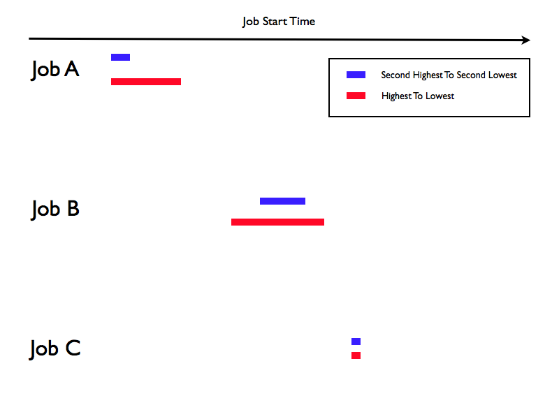
Consider:

This is, with the exception of the colouring, what my hack produced.

There are three jobs and I plot their start times, over a number of days. Actually I don’t: The red bars depict the earliest start time through to the latest. The blue bars depict the second earliest through to the second latest. In my test data I had five days of data so many jobs ran five times, some ran only once and one ran ten times. Next to the job name I print the number of times I saw the job run. (I also have a proper start time axis across the top.)

Though this is made up data the real data sample looked pretty similar:

• There were many jobs much like Job A and Job B, with lots of variation in start time.
• There were some jobs (mainly towards the front of the schedule) like Job C – with very little start time variation.

I think in the fullness of time I can do much better: This prototype uses Bookmaster Schedule tags to create a Gantt Chart. It’s monochrome and I think I’ve almost exhausted what it can do. But it was quick to code up and illustrates a point: Visualisation of job run times can be helpful.

The raw data is, of course, SMF Type 30 Subtype 5 Step-End records – and for once I didn’t need to change how the performance database is built. So the new bit is just more REXX code.

Futures

There are at least two things I can think of that would be better visualisations, though creating the apparatus to graph them would be a bit of a challenge. So I mocked up two possible graphs. While these graphs are almost identical they bear no relation to the one above.

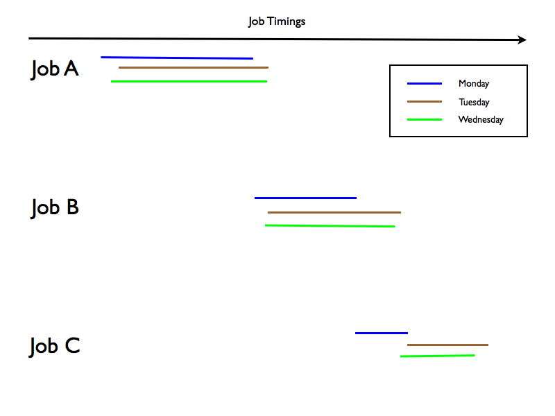
The simpler, and perhaps more consumable one in practice is:

In this one I plot both the start and end times for each job’s runs, with a different colour bar for each day the job ran.

This could show you the variance in start times and in end times.

It might be possible to produce it using bar charts with clever usage of invisible bars in the stacks but marking hours and minutes on the axis would be a nuisance. It might be easier to generate some HTML5 Canvas code (javascript) to create the whole thing.

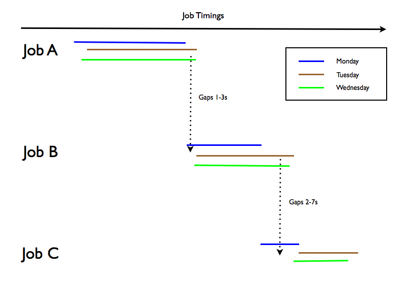
Now consider an enhancement – which in practice might get messy:

In this example the code would calculate the gaps between e.g Job A finishing and Job B starting and annotate the picture with it.

The calculations (as I mentioned in Games You Can Play With Timestamps) are very easy.

My concern about this is that the number of “gaps” annotations on a picture like this would grow to be huge very rapidly. Maybe some “smarting” that only annotates if the gaps between 2 jobs tend to be less than 5 seconds would help here.

It’s too tempting a goal to abandon entirely. And I can think of other wrinkles like annotating when jobs are consistently seen to start together.

But after a good day’s hacking I returned to the day job: A large mount of (non-batch) performance data arrived and duly got built into databases. And I’m looking forward to gaining insight into that customer’s systems over the next few days. But Hackday X was a great chance to explore some of the themes in (you guessed it) Games You Can Play With Timestamps which had been rolling around in the back of my mind. (You can imagine maintaining discipline to focus on less speculative stuff until Hackday itself was quite difficult – but I managed it somehow.)

But then that’s what Hackday is all about: Releasing untapped ideas into the wild and building prototypes that can be built upon later. If you ever get a chance to do something similar in your company do take it – it’s very rewarding but frustrating in that you only get a little time.

(Originally posted 2012-10-10.)

Round about now you’d be expecting posts to be geared towards the recent zEC12 announcement, or perhaps CICS TS 5.1 or the DB2 11 Preview, or IDAA V3. So what this post is about will probably have slipped by unnoticed. After all you don’t spend all your time looking for obscure New Function APARs, do you? 🙂

But I think some of you will find this one of value, or at least quite interesting.

(I presented a slide on this at the UKCMG 1-day meeting, October 10 2012, so you might consider this to be the script for that slide.)

I could’ve given this post a provocative title like "Do You Really Need CICS PA¹?" and you’ll see why that’s an only slightly daft question to ask in a minute.

Single TCB (task) speed has always been an important topic, and continues to be so. Here are three examples of why, irrespective of processor technology:

• For CICS regions much of the work is still performed on the QR (Quasi-Reentrant) TCB. There’s one per CICS region and when it’s saturated the region can support no more throughput: Installations are usually forced to split the affected regions.
• For CPU-bound batch jobs there is usually a single TCB conditioning their speed: To make them go faster takes application code tuning, removal of queueing or a faster processor.
• For complex CPU-bound DB2 queries the picture is similar to that of CPU-bound batch jobs. But here CPU Query Parallelism might help.

And these are just the most obvious examples, which we all know and love.

There’s an industry trend that’s beginning to make this even more important: Although the zEC12 had a very healthy single-processor speed increase over the z196, this is not a long-term trend. Processors of all architectures are getting faster more slowly, and this probably isn’t going to change. All architectures are relying on more engines and more threads to support larger workloads and zEC12 upping the limit to 101 engines from 80 is a good example of that.

So it behoves us to understand the single-TCB proclivities of our workloads, for all four reasons, and more.

A key point is, of course, what to do about it. But this post introduces some new instrumentation that at least helps with the analysis.

APAR OA39629, available for z/OS Releases 12 and 13, has the title "New Function To Report The Highest Percent Of CPU Time Used By A Single Task In An Address Space".

It provides two new fields in SMF 30 Interval (subtypes 2 and 3) and Step-End (subtype 4) and Job-End (subtype 5) records:

• CPU % of the highest CPU consuming task.
• This task’s program name.

For Step- and Job-end records the CPU % is highest percentage among the intervals during the running of the job or step.

The rest of this post is slightly speculative, as I’ll confess I haven’t actually seen SMF 30 records with the new fields in yet.

When there is no CPU you get blanks for the program name. If the program can’t be determined you get ‘????????’.

Let’s return to CICS: Consider the following diagram

This depicts a CICS region, though not a wholly typical one. As depicted, I would expect for most CICS regions the QR TCB to be the biggest. I don’t know whether the program name will actually be "DFHSIP" but I would expect it to be mnemonic and it’ll probably start with "DFH". If this is right we have a ready way in Type 30 to figure out how big the QR TCB is and therefore whether it is an impending constraint. And we can do this without creating CICS Statistic Trace records.² I mentioned Type 30 records and QR TCB in He Picks On CICS without a solution to the question of how to distinguish QR TCB from the rest.

The diagram also shows a File-Control TCB (think “VSAM”), three MQ TCBs and four DB2 TCBs. A typical region wouldn’t have all these doing much, if indeed they were present. And showing this level of evenness would, I’d hazard, be unusual.

For CICS regions with a heavy DB2 component, for example, the QR TCB might not be the biggest TCB³. In this case we’ll see a different program name and we can provide an upper bound on the QR TCB %. We’d do this by subtracting the biggest TCB (whatever that is) from the headline TCB time – also in the Type 30 (with some adjustments to make the maths right)⁴.

Of course CICS PA and the standard DFHSTUP (CICS Statistics Utility Program), which prints CICS TCB percentages at the subsystem level, do far more than just reporting CPU at the transaction instance and region level. But sometimes all you need is to figure out if the QR TCB is a vulnerability. In fact if you do have a region that needs work you probably would drill down (using something like CICS PA).

The above would use the Interval records (subtypes 2 and 3) and the same approach could be used with any long-running address space⁵. But there’s value for batch jobs – using subtypes 4 and 5. Admittedly most jobs are single-tasking. But not all are: For example, DB2 Utilities can be significant multitaskers⁶. So there is some value in finding the biggest TCB (and subtracting from the "headline" TCB number): You can better assess the benefit of faster engines (or understand which job steps are susceptible to engines not getting much faster).

So, I’m really looking forward to seeing real customer data – which I’m convinced will be very interesting.

I can’t believe it’ll be long before I see some. And when I do I’ll write some more about it.

Notes:

1. CICS Performance Analyzer, which produces reports based on SMF 110 Monitor Trace records. i.e. at the Transaction ID or transaction instance level.
2. I think this is actually quite significant: While I see customers with only a few CICS regions I see others with tens, hundreds or (in a few cases) thousands of CICS regions. Turning on Statistics Trace for a large subset of regions, particularly with a sensible Statistics Interval, is cumbersome if you’re just monitoring QR TCB %. Triaging them into "fix now", "monitor growth" and "don’t worry" regions is something you’d like to do with SMF 30 rather than SMF 110. After all most customers have SMF 30 Interval records permanently switched on.
3. I think this is a little unlikely: A CICS region will typically have multiple DB2 (or MQ) Attach TCBs, each of which would normally be quite small. So I’d still expect the QR TCB to be the biggest.
4. Another approach might be to use the fine structure of the Usage information I mentioned in Another Usage Of Usage Information. But the boundaries of usage might not completely align with TCBs. This is an experiment yet to be performed.
5. But many address spaces are architected so as not to have a "dominant" TCB, and indeed CICS has moved that way.
6. You could use SMF 101 Accounting Trace to see some elements of multi-tasking but I’d hope you wouldn’t have to.

(Originally posted 2012-10-04.)

I don't know how many of you will've spotted this but there was a nice instrumentation enhancement in the recent System zEC12 announcement.

It comes with the RMF support for CFLEVEL 18 (OA37826 and provides much more detail on paths to Coupling Facilities (CFs).

Previously RMF reported channel path acronyms – one per path. And that was all. (A channel path acronym is something like "CIB" for "Infiniband".) Those of you who know something about Coupling Facility link technology will recognise there are multiple types of Infiniband link now. If you do you'll equally recognise other deficiencies in the RMF topology information. This support fills in many of the gaps.

(Note: The existing support covers not only paths between z/OS LPARs and CFs but also between CFs – in support of structure duplexing.)

Though my personal interest is in the enhancements to the SMF Type 74 Subtype 4 record cut by RMF, there are corresponding enhancements to RMF Monitor III and the RMF Postprocessor.

So, what do we have?

• CHPID
• PCHID – which allows a better view of sharing where two or more z/OS images share a link to a CF. (This might explain why IC links don't play.)
• Channel Path Operation Mode – e.g. "CIB path operating at 1X bandwidth using the IFB protocol, adapter type HCA3-O LR". I hope you'll agree this is much better characterisation than just "CIB".
• Host channel adapter ID and port number.

The above is all topology information. What we don't have is traffic over the paths. Personally I think I'd like to see it for two reasons:

• Though I don't want to reverse-engineer path selection logic I do get questions about mixed topology z/OS-to-CF configurations and I'd like the data to provide answers on how traffic is routed.
• I'd like to be able to monitor path degradation – to proactively resolve issues. I'll admit the one "bad path" situation I've been involved with was catastrophic – in that the fibre broke – but seeing degradation over time would be useful.

If you agree that traffic and error analysis would be something you'd value let me know. Alternatively, if you think it's a dumb idea let me know (gently). 🙂

The new information is available for both z/OS-to-CF and CF-to-CF links. The only difference between the two is the "anchor" in the Local Coupling Facility and Remote Coupling Facility sections.

There is some performance information, which I think is useful:

• Path Is In Degraded Mode flag. This is binary and is passed from the hardware. I'm still getting clarity on what it actually means. What is clear is that there are both "path is degraded but some signals are getting through" and "path is totally dead" situations that could lead to this flag being set.

• Channel Path Latency Time. RMF uses this to estimate signalling distance at 10 microseconds per kilometer. Call me nosey but I really want this – as I like to figure out whether machines are close together or in different data centres.

  The field description notes this is the average round-trip path time in microseconds. A value of 0 means that the time was not measured. A value of 1 means a time less than or equal to one microsecond. So it's obviously not accurate enough to calculate distance to the nearest metre. I suspect we'll get to one of three states: The machines are very near to each other, they are a few hundred metres apart, or they are some kilometers away (and how far away they are).

Most of the information in the SMF record is in a new section (Channel Path Data Section) – which is going to cause mass bustage of my code. (Actually I don't handle Remote Coupling Facility sections terribly well so some reworking of my code is overdue anyway.) Fortunately the lab sent me a pretty complex set of data – so if I'm quiet 🙂 you'll know I'm 'heads down' in my code.

And I'm looking forward to seeing data from real customers: If you're at z/OS RMF Release 12 or 13 you can install the PTFs and take advantage of the new stuff too.

(Originally posted 2012-09-29.)

Do you see what I did there? 🙂

On March 10th I published the slides to “I Know What You Did Last Summer” on Slideshare. Since then I’ve given the presentation thrice and in the process got to know it a little.

(Yes I really do think creations take on a life of their own, sort of autonomously.) 🙂

So, six months on, I’m very pleased to have been asked to give the presentation again, but there are a couple of extra challenges in there:

1. It has to fit into 45 minutes, instead of 1 hour+.
2. It’s got to be sufficiently different to how it was before.

I’ll confess challenge 1 is one I should’ve addressed from the outset: You always have to be able to adapt your material to any timeslot. Yes, I can rip slides out but a “controlled contraction” would be better.

The second challenge is a blessing in disguise. The rest of this post more or less says why – and points the way to some future blog posts…

Much has happened in the past six months, some of which has been remarked upon in this blog. So the new elements I’m going to introduce are:

• Enhanced Coupling Facility Path-Level Instrumentation in RMF with CFLEVEL 18 on zEC12.
• What I’ve learned from the Usage Information in SMF Type 30.
• OA39629: NEW FUNCTION TO REPORT THE HIGHEST PERCENT OF CPU TIME USED BY A SINGLE TASK IN AN ADDRESS SPACE

The second of those I’ve already talked about. The other two belong as blog posts in their own right. Maybe “1 blog post per slide” is a good rule of thumb here.

Two other things have happened in the past six months are:

• I now have a semi-official part time role in pursuing the case for better instrumentation and talking about what we already have. I’m not sure this should be in the presentation.
• Talking to several customers and IBM developers through the summer I’m even more sure “Batch Architecture” gleaning is vital to many enterprises. So I ought to emphasise that more.

So, as I say, updating the presentation is something I want to do. And to see if I’ve made a good job of it come along to UKCMG FREE Forum on the 10th October 2012 at The Magic Circle in London.

(Originally posted 2012-09-24.)

This was originally going to be a different post about VSAM’s SMF 64 record, based on a customer situation. But it’s morphed into something else: A round up of "recent" enhancements to the SMF 64 record.

"Recent" is a nice euphemism: Some of these enhancements are 15 years old. 🙂 But let’s start the story at (or at any rate nearer to) the beginning…

Back in the early 1990’s I’d written the kernel of what would become SG24-2557 "Parallel Sysplex Batch Performance". Subsequently a few chums and I started putting together what would become "PMIO" – some tooling around which the Batch Window Tuning offering of the same name was built.

Other people in the team built the VSAM pieces – mostly out of DFSORT steps with assembler E15 and E35 exits, but also SLR as the database and REXX for reporting. Essentially the code marries up SMF 30-4 (step-end), 62 (VSAM OPEN) and 64 (VSAM CLOSE) records.

And it came to pass that I inherited all this code…

I’d not been closely involved with the code before so there was the usual re-engineering effort: Understanding the code, working on the comments and a little reformatting. It’s good code but quite fragile. So the "getting to know you" piece is essential. It’s the same as for any code adoption.

So what has all this got to do with "new" stuff in SMF 64?

If it ain’t broke don’t fix it" applies here – especially given what I said about fragility. So adding stuff that would give additional insight was what drove me to open up the code…

The first thing I added was new with z/OS Release 12: CA (Control Area) Reclaim. There are two fields in support of this line item: They tell me if you’re using CA Reclaim for a VSAM data set and if you’re getting benefit. (Thanks to Scott Drummond for reminding me of this – in the context of my customer’s problem.)

It’s not embarrassing that I’ve only just added this. But here’s one that IS: 🙂 In 1997 in OS/390 Release 4 DFSMS introduced System-Managed Buffering (SMB). This enables you to, for example, enable VSAM LSR (Local Shared Resources) and control it.

(LSR is a big deal as it allows you to change the VSAM buffering scheme to a better one than high-level languages tend to support. Previously one might’ve used the Batch LSR Subsystem to do this.)

So SMF 64 has lots of information on SMB, such as whether the JCL specifies what SMB’s buffering approach will be, whether it leaves it to SMB and what that approach will be (ACCBIAS). And now, only 15 years late, I capture this information: It rounds out what one can say about a VSAM data set’s performance rather nicely.

As for the customer situation: It turns out I mixed up CI (Control Interval) and CA (Control Area) split statistics (I do know the difference) and, wrongly concluded CA splits was a real issue. What I really had was a program-driven load (not a utility) which was causing a huge number of Index CI (write) I/Os. I think the simplest fix for this is to use SMB to turn on LSR buffering with Deferred Write.

It turns out this client is using neither SMB nor CA Reclaim. But if you get to send me your data I will now spot how you’re using these – assuming it’s relevant to the overall story. And we’ll see how well it’s working for you.

(Originally posted 2012-09-19.)

Prompted by Troy Coleman’s article zEC12 and zIIP Processors I thought I’d write about how I see the future for zAAPs.

First, his article does a good job of covering the area. So I recommend you read it.

Troy mentions the “zAAP on zIIP” function – which allows zAAP-eligible work to run on a zIIP. It’s not news and it’s a good piece of function: It means you can fill zIIPs more readily, making them a better financial proposition than if zAAP-eligible work had to stay on zAAPs, segregated from zIIP-eligible work. The value of this will depend on which of the following three categories your systems are in:

1. Mostly zIIP-eligible work.
2. Mostly zAAP-eligible work.
3. A mixture of both.

I see customers in all three categories. Strictly speaking I should say “systems in all three categories” as this is an LPAR-by-LPAR and machine-by-machine thing. So, to evaluate its applicability you need to use the usual methods (and apply some of the thinking in zIIP / zAAP Capacity Planning).

Troy also quotes the IBM Statement of Direction on the planned relaxation on the use of zAAP-on-zIIP:

IBM plans to provide a PTF for APAR OA38829 on z/OS V1.12 and V1.13 in September 2012 to remove the restriction that prevents zAAP-eligible workloads from running on zIIP processors when a zAAP is installed on the server.

This gives new configuration choices – which ought to be helpful to a number of customers: I can imagine migrations on an LPAR-by-LPAR basis to zAAP-on-zIIP.

He also mentions the Statement of Direction that:

IBM zEnterprise EC12 is planned to be the last high-end System z server to offer support for zAAP specialty engine processors.

So there’s an obvious direction of travel here. All these things taken together suggest the zEC12 timeframe would be a good one to migrate to zIIPs in. Actually I see nothing here that suggests you couldn’t do it on a z196 : Each customer will have their own choreography.

One final thing to watch out for: The configuration rules haven’t changed in that it’s still only one zIIP per GCP (General Purpose CP) and only one zAAP per GCP. There will be relatively few customers who need more zIIP engines on a machine than GCP engines (even with zAAP-eligible workload running on the zIIPs) but I’m sure they do exist. In those cases careful evaluation (particularly of the financial kind) will be the order of the day. And that’s where Capacity Planning, mentioned in my referenced post, comes in.

(Originally posted 2012-09-18.)

I’ve written extensively in the past about what you can glean about batch suites from SMF, most notably SMF Type 30.

While I don’t believe SMF alone can give you the full dependency network (complete with validation) I’ve just added some analysis to my code that gets me a little closer. As you’re probably never going to run my code the bit that would be interesting is the kind of inferences it’s now drawing. You might want to duplicate and refine them.

I have a standard report for a suite (a group of jobs with a naming convention) that lists their start and end times (amongst other things). It was written in the mid 1990’s and did just fine for a while. In fact it never broke, it just got underwhelming. 🙂

Looking back at the change log 🙂 I see I made a major enhancement 2 years ago: The code uses Job Identifiers and Reader Start Times to attempt to find jobs released together. Doesn’t work as well as I’d like because it can take more than a second or two for a job to get released so many false negatives occur. But still it reveals (true) stuff.

The latest enhancement attempts to glean something from both start and end times for a stream of jobs:

I’m trying to figure out whether one job follows directly on from the previous one, whether it kicked off in parallel with it, or what.

So here are some tests the code performs, stopping after it satisfies any test.:

1. If a job starts no more than 5 seconds after the one above AND it starts before the one above finishes then I consider it starting together with it.
2. If a job starts after the one above finishes but no more than 5 seconds after it finishes I consider it a a follow-on job.
3. If it starts within the same minute that the one above starts I print an = and not the start time (as that would be tedious and unmnemonic). It might be a co-starter, but it might not.
4. Otherwise I print the start time as there’s some sort of a gap¹.

If you were to ask “is this rigorous?” I’d have to say “no”.

If you were to ask “is it helpful?” I’d say “yes”:

“In tests” 🙂 it’s illuminated what would otherwise be an impenetrable set of start and end times. In other words it’s helping me edge towards a better understanding of a group of jobs.

Now, suppose my code hinted at a dependency – the “follow-on job” case. It wouldn’t explain the dependency². There are things in SMF that might explain or corroborate a dependency: SMF 14 and 15 for non-VSAM data sets and SMF 62 and 64 for VSAM data sets can be used to understand some dependencies.³ If I see a “follow-on” case I’d be inclined to look at the jobs involved and their access to data sets. I wouldn’t be nearly so rash as to suggest the lack of “data set” dependencies means the jobs could run together.

In fact this illustrates something fundamental about the nature of batch: It’s very fragile and drawing the wrong conclusions is easy to do – with potentially disasterous consequences. Lots of people have started on batch analysis with the “how hard can this be?” attitude and ended up answering that with “it’s actually very hard”. It’s a steep learning curve but do get a helmet, a rope, crampons etc and start the climb. 🙂

With that climbing analogy I should say the point isn’t to reach the top (I don’t feel I have, for instance) but rather to make progress, lots of progress. In that vein, the algorithm I’ve explained above takes me quite a bit further. I hope you find it useful, and maybe you can provide fresh insight: My code continues to evolve as I spot patterns and things, which is exactly the way I like it.

---

1. By “gap” I don’t necessarily mean nothing ran but just that no jobs in the suite ran in that gap: In my test case I can see this suite waiting for other suites to get to a certain point.
2. And nor would the scheduler’s schedule: It just describes the dependencies as the installation saw fit to identify them,
3. DB2 data access is a notable case where SMF won’t tell you about the dependency.

(Originally posted 2012-09-13.)

This post is about unusual ways of using the SMF 30 Usage Data information, some of which you’re certain to want if you’re managing z/OS systems’ performance.

A long time ago I noticed character strings in SMF 30 records that looked like product names. (As is my wont I was looking at the raw Type 30 records for a different purpose and spotted them.)

Some time later I figured out these were Usage Data sections. And the strings were indeed product names, but there’s much more besides.

Here’s an example:

Suppose you wanted to know which address spaces were CICS regions. (I do, when conducting a study, but you may feel you already know.) Well, finding address spaces with a program name of "DFHSIP"¹ gets you that far. But here’s a nice twist:

Suppose your installation was in transition from CICS 3.2.0 to CICS 4.1.0. Without asking anyone about progress you can use the Usage information: The string

IBM CORP        CICS            V3 R2.0 DFHSIP  5655-M15

tells you all you need to know.²

The same is true for DB2, Websphere MQ, Websphere Application Server, TSO and IMS³, amongst others.

Other companies’ products are represented in the data. In one case the Product Version is "**.**.**". As I mentioned in ³ I think it’s z/OS doing the formatting and in this case overflowing.

By parading IBM products and mentioning other companies’ products I don’t mean to suggest all products use the IFAUSAGE macro to REGISTER. Indeed, support has evolved a little in the products over time. The next example will illustrate this.

Suppose you wanted to know which DB2 subsystem a CICS region connected to, again without asking anyone⁴:

Recent levels of DB2 will – in their Product Qualifier field show you the subsystem name:

IBM CORP        DB2             9.1.0   DB2T    5635-DB2

But I have at least one set of DB2 Version 8 data without the equivalent of "DB2T" in it. So DB2 has changed to provide more information.

So far my examples have been "online" rather than "batch". They happen to be taken from SMF 30 Interval records (Subtypes 2 and 3). There’s a nice use case for Batch, though:

The Step- and Job-End SMF 30 records (subtypes 4 and 5) also have the product information. If I know a jobstep is “TSO”⁵ and I want to know if it calls DB2 I can look in the Usage information. Here’s a real Version 8 example:

IBM CORP        DB2             8.1.0   NONE    5625-DB2

Until I was armed with this information I assumed all TSO steps were DB2 steps. In reality they could be something like REXX execs (which most of my programs are). Now, you could use DB2 Accounting Trace (SMF 101) to sort this out – but why bother?

One thing is puzzling me with this data – and at first I thought it was a bug in my code:

I see in at least two cases⁶ duplicate Usage sections. These aren’t 100% duplicate – the 5 character fields are all the same but the numeric fields differ – but very similar. I saw a CICS region with many dozens of MQ Usage sections. Each had different numeric values. Further, the number of these varies from interval to interval for an address space. An oblique comment I read got me thinking: The comment included the term “TCB”. So I speculate that each of these quasi-duplicate sections represents a TCB or SRB⁷ or something like that. Can you, dear reader, clear this up?

So those are the things I’ve already figured out I can do with this information. My code at present just works with the Interval records but I can easily extend it to Subtypes 4 and 5. And it only records 4 sections per record. Again I can easily extend it. I pick up the section count, for the reasons outlined above. You might be wondering about the data’s original purpose:

Given that each Usage section includes TCB time and SRB time I would expect people would be using to charge back at two levels:

• Charging for using a product e.g. DB2 (but probably not down to the subsystem level as that’s a little more obscure).
• Charging for using a product based on TCB and SRB time.

But that’s just my expectation. I’d like to know what you use the Usage Data section information for, if you do.

---

• ¹ I’ve already mentioned this in CICS and Batch, What’s In A Name? and He Picks On CICS.
• ² This is in fact five adjacent fields in the record – Product Owner, Product Name, Product Version, Product Qualifier and Product Identifier.
• ³ For IMS Version 11 the Product Version string is an unexpected "V1R1" which leads me to suspect z/OS is doing the formatting.
• ⁴ As usual the maxim is "don’t ask people for information you can get from system instrumentation".
• ⁵ This would be if the program name was something like “IKJEFT1B”.
• ⁶ CICS / MQ and DB2 Stored Procedures.
• ⁷ Whether this is a case of “ever existed in the interval” or “existed at the end of the interval” I don’t know.

(Originally posted 2012-09-06.)

I hope you like my new blog banner – in honour of the new zEnterprise EC12.

We actually announced the zEC12 (for short) the day I returned from vacation. Great planning, IBM! 🙂 It’s taken me a while to catch up – and changing the banner was an important step. 🙂

I’ve known about the soon-to-be-announced processor range for quite some time, as I think you’d expect. And tracked what was going to be announced quite carefully. The trouble with tracking something to announcement is you lose some of the “surprise!” factor – which I used to quite like back in my younger days.

I won’t precis the announcement details here. But suffice it to say the zEC12 is improved compared to the z196 in almost every area.¹.

You could call it “evolution” rather than “revolution” but there have been a multitude of changes in places that matter. I’d like to highlight, though, a few qualitatively new features:

• zAware – which runs in a special LPAR and uses analytics capabilities to analyse system messages, providing an almost real time view of systems’ health. It learns from the message traffic patterns, using the information to identify unusual system behaviour and minimise its impact. It’s based on technology from IBM Research.
• Flash Express – which some people have commented looks like a rerun of Expanded Storage. Personally I’ve seen a number of nasty customer situations where this would’ve really helped out. I’m thinking of when systems have to capture a dump at just the wrong moment – or into already over-committed memory/paging subsystem configurations. I’d like to think it would be equally useful for the happier times, too – such as workload bursts and batch/online transitions.
• CFLEVEL 18 – which has many enhancements. For me the one that caught my eye was the enhancements to path statistics, externalised through RMF. I’m going to write a post on this some time. (I believe this one, though part of the announcement, is retrofitted to z196. I hope so because I’d like to see customer data with these new fields in from older machines than the zEC12.
• Transactional Memory – which is aimed at increasing concurrency for applications that use a shared set of data. As we go to higher numbers of processors and degrees of concurrency this sort of thing becomes increasingly important.

This obviously isn’t an exhaustive list but it gives you a flavour: Each new processor range is more than just faster / higher capacity / better environmentals.

For much more detail read the two Redbooks:

• IBM zEnterprise EC12 Technical Introduction
• IBM zEnterprise EC12 Technical Guide

The team that wrote these excellent Redbooks includes a number of friends of mine. I found the books a very enjoyable read. Note: They are still in draft.

---

1. One exception – which I really don’t think will affect many customers – is maximum memory: It stays at 3TB.