(Originally posted 2013-01-21.)

To me learning is like Microwave Popcorn.

Specifically, turning

into

Part of the fun of making popcorn is watching the bag and listening to the poppings: As each kernel pops it pushes the bag out.

And so it is with learning: Every piece of knowledge contributes to the overall shape.

Anyhow, enough of the homespun “philosophy”. 🙂

I was maintaining some ISPF REXX code recently and it caused me to come across two areas where REXX can really help with ISPF applications:

• Panel field validation.
• File Tailoring

The introduction of REXX support is not all that recent – I think z/OS R.6 and R.9 were the operative releases – but I think most people are unaware of these capabilities.

I’m not an ISPF application programmer so if you want the technical details look them up in the ISPF manuals. But here’s the gist of why you might want to consider them.

Panel Field Validation

On one of our ISPF panels we have eight fields that together represent a time/date range. You can (with VER(), as you probably know) check these fields – two sets of year, month, day, hour, minutes – have numeric values and aren’t blank. I don’t think you can check things like whether the end date is after the start date, or whether these two dates are before today. For that you need REXX:

With *REXX in the )PROC section of the panel (terminated with *ENDREXX) you can inject REXX code. If you set variable zrxrc to 8 (and set zrxmsg to an appropriate ISPF message number) you can fail the validation. If you set zrxrc to 0 you can pass it.

Of course you might be in a position to do this all in the REXX that causes the panel to be displayed in the first place. But there are two reasons why I think you’d want to do it in the panel definition itself:

• It’s a lot simpler than having the driving REXX redisplay the panel if the fields don’t validate.
• Keeping all the field validation logic together – VER() and REXX – is much neater.

But you have the choice.

File Tailoring

Again driven by REXX, the code I maintain uses ISPF File Tailoring to create JCL from skeleton files, based on variables from ISPF panels.

You can write some quite sophisticated tailoring logic without using REXX. But with REXX you can do so much more.

(My first test case used the REXX strip() function to remove trailing blanks. Of course you can do that with )SETF without REXX.)

If you code )REXX var1 var2 … then some REXX then a terminating )ENDREXX you can use the full power of REXX.

In the above var1 etc are quite important: If you want to use any of the File Tailoring variables (or set them in the REXX code) you have to list them.

Note: You can use say to write debugging info to SYSTSPRT.

I don’t believe you can directly emit lines in REXX but you could set a variable to 1 or 0 and use )SEL to conditionally include text.

Again, you could perhaps do some of this in the REXX that calls File Tailoring. But I’d prefer as much of the generation logic as possible to be in the one place: The File Tailoring skeleton. This is particularly true of variable validation when you consider you can use )SET in the skeleton to set the value of a variable – after the validation code has run.

---

So these two items – panel field validation and file tailoring – were areas I unexpectedly found myself researching. I won’t claim they’re core to my “day job” or particularly profound but certainly they proved handy. If you find yourself developing with ISPF facilities they might save you a lot of time.

And certainly I feel my grasp of ISPF is that much better – but maybe because of the 2000 lines of ISPF REXX I reformatted and adopted in the process. 🙂

(Originally posted 2013-01-13.)

First, a belated Happy New Year! to everyone. It’s been a busy past few weeks, not least because of the customer situation I’m working on.

But, to kick off 2013 here are the two conference abstracts I submitted for the UKCMG Annual Conference. No pressure, guys. 🙂




Time For DIME

In recent years memory has become cheaper, or certainly more plentiful. This enables us to do new things, or old things faster and better.




I believe it is indeed Time For DIME (Data In Memory Exploitation). But we’ve been here before – in the late 1980’s. Much has changed but the basic concepts haven’t. So this presentation reminds us of "the way we were" but brings things right up to date. It covers why you’d want to run a DIME project and how to go about it: It covers both the project phases and technical aspects, preparing you to make a quick start on realising the benefits of DIME.




While the main example presented here is DB2, the presentation also discusses Coupling Facility memory exploitation, as well as a number of other examples.

The Life And Times Of An Address Space

A typical z/OS system has a wide variety of address spaces. So much so that managing their performance can be difficult.




This presentation prepares you to handle this diversity, discussing what’s common to all and what’s different. Centred around SMF Type 30 records, it guides you in deciding when to rely on common instrumentation, and when to go to more specific data, such as CICS instrumentation or data set records.

 

---

Personally I find it very difficult to write abstracts – particularly as you end up trying to write them before you write the actual presentation. So the finished result can be different. But then every time anyone ever gives a presentation it turns out at least a little different.




As for the UKCMG Annual Conference, this is an event I’ve been proud to present at most years in the last 20. It’s always been a great crowd and a good opportunity to catch up with what people are doing. This time it’s in London at the CBI, instead of being out in the country. I don’t know how much difference that will make. Come and join us if you can. Here’s the link: UKCMG Annual Conference, London, May 14-15, 2013

And a final thought: I write about what I want to write about (and what I think is important). If you have ideas of what I should be presenting on and writing on do let me know.

(Originally posted 2012-12-11.)

There was a time before blogging 🙂 and what I’m about to talk about is something I used to explain quite often back in those days.

Reminded by a current customer situation – and needing to explain it again – I thought it time to do it this way.

(Here I’m presenting a simplified view, but one that covers the salient features that might help you.)

The CICS / DB2 Connection code provides a number of possibilities for optimisation, one of which is Thread Reuse. This post won’t discuss the mechanics of this in any depth but aims to explain the effect of it on DB2 instrumentation – in fact DB2 Accounting Trace (SMF 101).

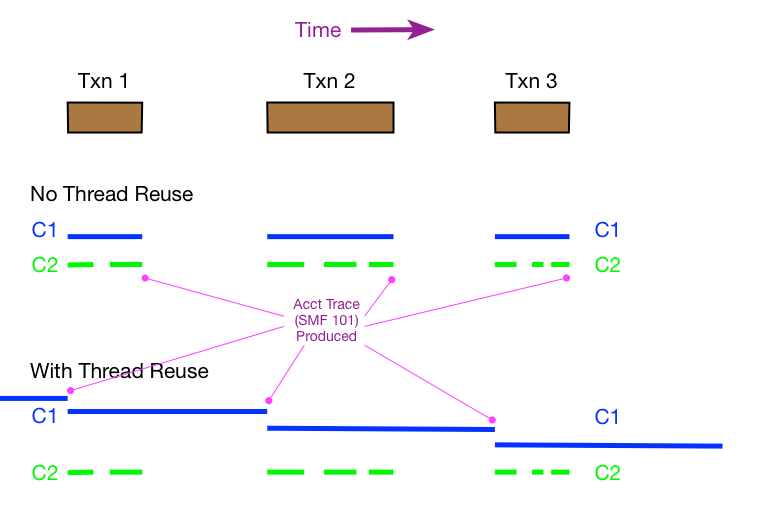
Consider the following diagram, with time flowing from left to right…

I’ve shown the two scenarios one above the other. Blue bars represent periods of Class 1 elapsed time. Green bars periods of Class 2 elapsed time. Notice how the blue bars are unbroken but the green ones can have gaps: Because Class 2 represents the time actually in DB2 there can be time between “stanzas”. (But SMF 101 doesn’t record the timings of the gaps – just two numbers which when subtracted give you the total time.)

The diagram shows three CICS transactions running one after the other, with Thread Reuse and without:

• In the case without Thread Reuse three threads have to be created and terminated, one after the other. This is an expensive process, which is why Thread Reuse is used.
• In the Thread Reuse case the thread is reused twice, avoid the thread management lifecycle.

The reason for discussing this is that with Thread Reuse DB2 timings in Accounting Trace (SMF 101) work a little differently.

(One thing that remains unchanged is the relationship between Class 2 elapsed time, Class 2 CPU time, the Class 3 wait components, and what’s not accounted for but still part of Class 2 elapsed time. So I won’t discuss those here. What’s also not changed is Class 1 CPU time – so computing Non-Class 2 CPU time is the same – Class 1 CPU minus Class 2 CPU.)

The most important thing to notice in the diagram is the difference in Class 1 time behaviour:

Instead of – as with the non-reuse case – starting and ending at the transaction boundaries, Class 1 time now ends when the next transaction that uses the thread starts. (And that’s when the DB2 Accounting Trace (SMF 101) record is produced.) This means, as you can see, a lot of the Class 1 elapsed time has nothing to do with executing the transaction. Obviously, under these circumstances, you can’t use Class 1 elapsed time for much.

An obvious question is “when can you trust Class 1 time in a CICS environment?”

Fortunately the answer is quite simple: The value of a field in the 101 record (QWACRINV “Reason For Invoking Accounting”) determines whether you can.

If QWACRINV has a value signifying either “New User Signon” or “Same User Signon” you know the thread was reused. Otherwise – probably with the value signifying “Deallocation” – you know it wasn’t.

(If you wanted to know how effective Thread Reuse was you’d calculate – as my code does – some ratio relating these two Signon values to Deallocation.)

In the case I’m dealing with some of the transactions in the CICS region use Thread Reuse and some don’t. For those that do I’m discarding the Class 1 elapsed time and for the rest I’m using it to give some understanding of the timings outside of DB2.

I have to be very careful when I say “some understanding of the timings outside of DB2” – but that’s really a topic of a completely different discussion, involving things like Unit Of Work Identifiers. (CICS PA does a nice job of bringing it all together – to the extent it can be.)

For now I wanted to explain why I’m careful in handling DB2 Class 1 Accounting elapsed times for CICS transactions. And to socialise a briefing for friends of mine. I had honestly aspired to be brief – and it’s frightening to me how much detail I’ve left out – but brevity was not to be.

(Originally posted 2012-12-09.)

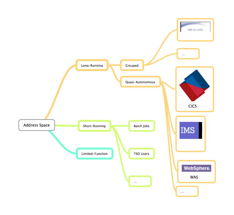
I’m trying to put some structure on the idea of Life And Times Of An Address Space. The best way to do it, I think, is to attempt a taxonomy of address space types. So here’s an initial stab:

One thing that immediately comes to mind is you can map useful SMF record types onto it:

Three things:

• I think it immediately betrays my bias towards SMF 30 in what I get to write about. But I think that’s the point: Making instrumentation tell useful stories.
• I haven’t attempted to draw in the product-specific instrumentation. I may well do so as another point of the presentation is likely to be “to get really useful you sometimes need to go to product-specific stuff.
• On a technical note, batch jobs run in initiators – which are typically long running. In fact (e.g. with WLM-Managed Initiators) this might not be the case. In any case I think this is a useful simplification that might survive this writing process.

At this point the purpose of publishing this “0.0” version (as you’d see from the URLs of the two pictures) is in case someone says “you’ve got the taxonomy all wrong” or “I don’t like the direction you’re headed in. Though you might find it a useful taxonomy all in its own right.

Yes, I know the annotation is unsubtle. It’s an experiment with Skitch annotation. Of course my home-grown HTML5 Canvas annotation code is much nicer. 🙂

And the product logos are also probably not the final ones I’ll end up with: They’re really my first go at adding graphics to a MindNode-produced mind map. (And I’ve not tried using MindNode for taxonomy before.)

Still, it’s better than a beer mat. (Who am I kidding?) 🙂

Now, if you were to annotate either graphic and send it back to me that’d be interesting, dontcha fink?

(Originally posted 2012-12-08.)

Every year I like to debut one new presentation, though that isn’t a firm rule: In 2012 I debuted “Send In The Clones” (SITC)¹ and “I Know What You Did Last Summer” (IKWYDLS), but actually only the first one was written in 2012.

Of course presentations are “slow trains coming”: I widely trailed my desire to write IKWYDLS in 2011 and finally revealed it early this year. (In fact it evolved through the course of the year into “I Know What You Did THIS Summer” and I now refer to is as “I Know What You Did This Last Summer”.) 🙂 Or “IKWYDTLS” for short.

SITC arose much more spontaneously – being initially a presentation for a customer working group. (And it still has some of that genesis in it – with a rather pointed “where from here?” slide left in.)

The point of the above is generally I don’t just get up one day and decide “today I’ll put on a show”: You have to “record” before you can “gig”. (Of course I do just say stuff sometimes.) 🙂

So what about 2013?

I have two ideas swirling around in my head, and I’d like to know if either appeals to you:

1. Time For D.I.M.E.
2. The Life And Times Of An Address Space

Time For D.I.M.E.

This is more a “campaign” presentation in that I really do think it’s time (judging by my customer set) for customers (particularly those running z196 and zEC12 machines, but also z114) to consider memory usage afresh. (DIME is, of course, short for Data In Memory Exploitation.) (With the advent – a while back but practically into 2013 – of DB2 Version 10 this becomes even more relevant.)

This is probably the presentation my management would be keener I wrote – though it’s one I personally feel strongly about anyway.

The Life And Times Of An Address Space

I like to write occasionally about more abstract things, things with less immediate punch in their message. This presentation is very much in that category. Its origins are, I think, the lower-level pieces of IKWYDTLS. When giving that presentation I had to gloss over the address space piece. And there was so much more I wanted to say than was even on the slides. And stuff has happened this year that makes it even worse – as regular readers of this blog will know.

I also think there’s something of a (pseudo-)intellectual framework to be espoused here: For example, we can view batch jobs and CICS regions as looking very different but actually there is much commonality. I’d like to explore that.

(There is a practical benefit as it’s important to use the commonality but respect the differences when designing reporting.)

I also think it’s important to get beyond the idealised address space and into practical examples, such as CICS and DB2.

(Somehow BBEdit, which I’m writing this in, seems to have learned to prompt me with the words “CICS” and “DB2.) 🙂

So How About You?

What do you think of those two ideas? Feel free to comment here or in any other way you like. The aim is to take these two ideas (and any others) and turn them into useful material, whether actual presentations, blog posts, analysis code or whatever.

The next step is probably to inflict more of my handwriting on you. 🙂 And, as I’m not so good at graphics, I might collect some napkins from around the world to draw them on and post photos of these rough drafts as we go along. 🙂 Now wouldn’t it be fun to do a presentation composed entirely of photos of drawings on interesting pieces of paper, sides of cows, people holding placards² etc? 🙂

---

Notes:

¹ Queen fans tend to refer to songs and albums by obscure sets of initials, so that “TMLWKY” is “Too Much Love Will Kill You”, “NOTW” is “News Of The World” etc.. TMI? Perhaps. 🙂

² I see CICS has already done it. 🙂

(Originally posted 2012-12-04.)

I’ve talked about BPXWUNIX before but here’s a nice use case: Filtering REXX query results.

When I get your performance data I have code that stores it in a database which I query with (essentially) REXX. The predicate syntax is very simplistic so I’d like to do better. I can’t replace the syntax (not entirely true but close enough) but I can filter the results better.

Consider the following single step:

Reading it as a "U" shape, I pass the query results to a Unix Pipeline consisting of two stages:

1. grep – which filters the query results, prepending the all-important line numbers
2. cut – which removes the line contents, leaving just the line numbers

These line numbers (stdout) are passed back to the REXX driving code, along with any error information (stderr).

Any use case would be expected to check stderr before processing stdout.

But what is the point of jumping through these hoops?

As I mentioned most recently in Towards A Pattern Explorer – Jobname Analysis , regular expressions (regexps) are very flexible. So I can very easily code a filtering regexp that could be used to reduce the results of my original database query. The diagram above shows just such a workflow. But now for some actual REXX code…

/* REXX */ 
s.1.1=1234 
s.1.2=7543 
s.1.3=8911 
s.2.0=3 
s.2.1='XYZZY' 
s.2.2='Proxy' 
s.2.3='Xylophone'

atstart='¬' 
grepstring=atstart'XY' 

cmd='grep -i -n "'grepstring'" | cut -f1 -d:'

call bpxwunix cmd,s.2.,filter.,stderr. 

do f=1 to filter.0 
  item=filter.f 
  say item s.1.item
end 

do e=1 to stderr.0 
  say stderr.e 
end 

Let’s examine the code:

• The first few lines emulate the query – filling a grid of stem variables with data. The code filters on the s.2. variables but eventually it’ll be the surviving s.1. variables that will be printed.
• The line where atstart is assigned a value is interesting: With my emulator (x3270) I can’t actually type a circumflex (^) but it turns out the tilde (¬) works fine for me instead. (In regexps "^" means "the match starts at the beginning of the line".) So I set this variable so I never have to worry about it again – using it as I construct the regexp in the next line.
• In this example the regular expression merely says "match anything starting with ‘XY’". Big deal, I could’ve done that easily in REXX. 🙂
• The "-i" switch on the grep command says "match without regard to case". Again easy to do in REXX. 🙂
• Specifying "-n" says "add line numbers on the front of the matching rows.
• Cut throws away the matching rows, just returning the line numbers for them. "-f1" says "return the first field" and "-d:" says "the first field ends at a colon". In fact the line number ends with a colon so this is a good point to cut the record".
• Note that s.2.0 has to be set to the number of variables to be passed but s.1.0 doesn’t. I stress this as it may catch you out.
• Results are returned from BPXWUNIX in filter. variables (and filter.0 is the count of them) and stderr. contains any error messages.
• The first loop iterates over the returned results (two records in stdout, one with the number "1" and the other with the number "3"). These are used as indexes into the s.1. variables. So s.1.1 (1234) and s.1.3 (8911) are printed.
• Finally any error messages are printed. In Production you might actually test for the presence of nastygrams 🙂 before deciding to use the results of the grep / cut pipeline. In my testing I want both.

There are probably other ways of achieving the same thing – using regexps – using Unix programs. If you prefer them use them. This one seems quite simple to me, Unixwise. And it certainly complies with my performance objective of only transiting once to Unix programs and back. Of course, if you have a lot of filtering instances within a program you’ll transit more often – but then the effect on performance is probably still unnoticeable.

I think the first place I might use this is to better refine what I mean by a “Batch Suite”. I’ve talked about that one before.

(Originally posted 2012-12-03.)

Just a brief follow on to Bad Data And The Subjunctive Mood: Here’s a podcast I like to listen to while running. (Music and podcasts are about the only thing that keep me running, that and the success at my modest goals.)

BBC Radio 4 has a very nice programme More Or Less: Behind The Stats. It’s a magazine programme with extremely digestible yet thought-provoking items on Statistics.

My tendency with radio programmes in general is to think ahead to where they’re going next. Start The Week would be a good example (though I find it frustrating when they miss angles). Another good example would be Friday Night Comedy but for slightly different reasons. But for More Or Less they tend to throw in things that surprise me, more than they leave out things I expect them to say.

I’m not sure whether these podcasts are available worldwide or just in the UK. Perhaps someone can let me know. In any case More Or Less would be good for “Data” people.

(Originally posted 2012-12-02.)

Or should that be “Subjective Data And The Bad Mood”? 🙂

A good friend of mine says that when dispensing advice one shouldn’t use “may” or “might”, but that one should be more definite.

I’ve probably said this before: When I say or write “may” or “might” I’m deploying the subjunctive mood for what I hope aren’t “weasel words” reasons. My claim would be the subjunctive mood reflects some underlying subtlety like genuine reasons for doubt, and that I’d be forthright in standing behind this more nuanced position.

(I do sometimes catch myself saying “may” when I mean “might”, but I think we all do that.)

Now, to come to(wards) the point, I’ve been saying for a while now that “data provenance” is important.

So I see a field in a record which is acting bizarrely (as happened to me this week)…

• Do I conclude the field is broken?
• Do I conclude it’s telling the truth?
• Do I conclude it’s telling one version of the truth?

I think the sensible thing to do, rather than leaping to any conclusion, is to seek corroboration. But also situational context.

This latter point is actually quite important and one us technical people tend to forget… So what if MSTJCL00’s working set appears to be 2GB on every LPAR the customer has? (And this was the case this week.) The “so what” on this one is the obvious economic cost but also the sneaking suspicion that some other nasty effects are occurring. (Perhaps cruelly it might be worth noting the customer should’ve spotted this – if it’s a true phenomenon.)

I’ll also note that in my – nowadays wide and varied – experience of customer systems I’ve never seen MSTJCL00 be more than a few tens of megabytes. Indeed another customer’s data that I’m currently reviewing shows this norm in action.

I glossed over corroboration back there. It turns out the customer is also seeing the phenomenon – now they’re looking for it (I think using RMF Monitor III) – and will be pursuing it as a potential defect. Where that takes us I don’t know yet, it being out of my sphere of understanding.

But you can see that for me to barge into the customer and tell them that they’d better fix this usage of memory, without a hint of doubt, would not be the right approach. Working with them to establish the truth and its relevance is much better. So phrasing like “it looks a lot like you’ve got a problem worth worrying about with MSTJCL00’s use of memory” is better.

By the way in this case I suspect MSTJCL00 (Address Space 1) is an anchor for the storage and it may well be some other user of 64-bit Common that’s the real big user.

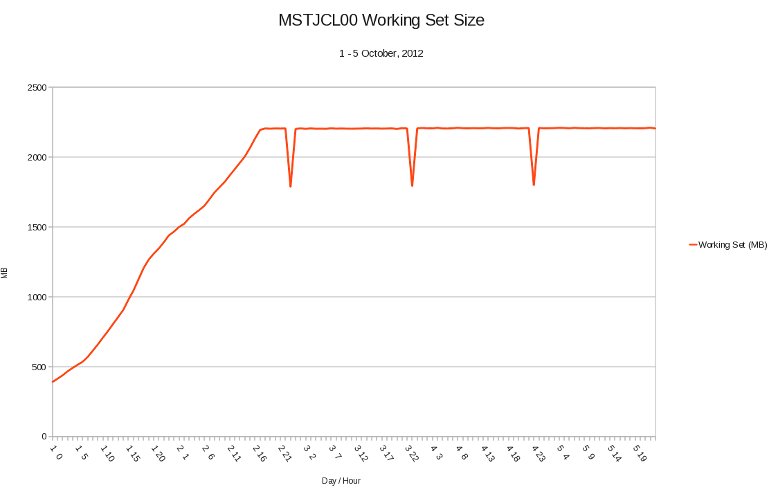
In case you think this might be bad data or at least an isolated bad data point look at the following graph:

The days and hours are along the bottom and the system was IPL’ed the day before.

There is something funny about the 11PM hour on each day (which might give a clue) but otherwise the picture is reasonably clear:

• The working set rises from a “normal” value just after IPL until it reaches a steady state.
• If this is a memory leak then something’s having to “bail out” to create the levelling off we see.
• As the final usage is more than 2GB this is either a number of 31-bit address spaces and/or dataspaces, or else it’s 64-bit. Personally I suspect the latter and that this is a 2GB large memory object filling up. But what?

So one of the points here is the value of a time-driven view.

Now for something approaching a “payload” for this blog post:

We have to be careful of the provenance of any data we use. And a very good book on the subject I’ve been reading is Bad Data Handbook. Whether you’re a data scientist (and I think very few of those would be following this blog) or a performance specialist it’s a very worthwhile read, being a collection of papers from many authorities on the subject. You won’t find anything specific to mainframe performance in it but the more general lessons are readily applicable. In general performance people need to take on board some of the data science lessons and this is a good primer.

(I bought my copy as a digital download: It seems O’Reilly have frequent 50% off deals and I took advantage of the recent one. There might be another one along soon.)

See what I did just there: I used the subjunctive mood (“might”) to alert you to the possibility. I think that was useful. 🙂

The point of this post has been threefold: To urge the correct use of “might” (and “may”), to mention this MSTJCL00 observation at a customer, and to mention the Bad Data Handbook. Comments on all of these are, of course, welcome.

(Originally posted 2012-11-24.)

I seem to be obsessed with finding patterns in data, don’t I? And, to my mind, I’m insufficiently obsessed to bring it all to a thunderous conclusion.

Pardon the self-flagellation 🙂 here: This stuff is technically difficult. But just yesterday I think I made a breakthrough. I think it’s worth sharing it with you. But first some motivation and some prerequisite knowledge.

Motivation

In one of my current studies I encountered a WLM service class with over 100 IMS Message-Processing Regions (MPR’s), a sea of address space names that all seemed to start with “IM” and had a “T” as the fourth character. I wanted to do two things:

• See how well this pattern fitted (and any others I thought I saw).
• Extract any varying portions.

As you’ll see with Regular Expressions I could do both.

Regular Expressions

Regular expressions (in this post referred to as "Regexps" though often seen as "Regexes" or "Regex’s") neatly (but geekishly) solve the problem of a general search and matching language).

Regexps are extremely powerful and reasonably well understood in the Unix / Linux / Web world. We don’t really know them in the z/OS world but we can certainly use them. Tools like sed, awk and grep all use Regexps. In my case I’m using the PHP built-in prey_match() function.

Consider the following regular expression: ^IM(.)T(.+)$.

It looks complicated, but let’s dissect it:

Believe me you soon get used to the above set of pretty standard pieces of RegEx.

This particular Regexp wasn’t chosen at random, or particularly to show off features. It’s actually the first one I used on real live jobnames – as I thought I saw a pattern.

Capturing groups need a little explanation – as they’re a very useful and highly relevant feature of Regexps. They have two main functions:

• Allowing you to extract the varying portions of the string being matched. This, you’ll recall, I wanted.
• Through the use of back references to refer to a varying match early in the Regexp in a later portion of the Regexp. For example, “\1” refers to the first capturing group. (I actually didn’t need this but it’s possible I might in some other set of data.)

I replaced the second capturing group – “(.+)” – with one that more tightly defined the match: “(\d+)” matches any number of numeric digits. The number of matches stayed the same, demonstrating that all the jobs had a trailing numeric identifier. (I’d suspected this but wasn’t keen on wasting my time checking it when a well-crafted Regexp could do it for me.)

So, I’ve shown you some of the power of Regexps. And they’re not too bad to work with once you’ve got used to them.

My Prototype

Bear in mind this is a prototype that’s already yielded results: I’m confirming patterns, counting matches and extracting variable portions of job names.

I wrote some PHP code, using the preg_match() built-in function to do the Regexp work. This code reads a file containing the results of a query against my performance database, each line starting with the SMFID and the job name. It also puts up an HTML form (the reason this is PHP) which allows me to enter up to five Regexps. These Regexps are all applied to each job name and a line printed about the job’s matching, including the fragments yielded by the two capturing groups.

A count of matches for each Regexp is printed at the bottom, together with the number of job names that failed to match any of the Regexps.

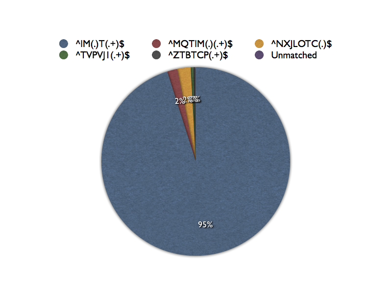
In fact with five Regexps only one job name failed to match. These five Regexps are disjoint in that none are refinements of any of the others. If I put them on a pie chart it would look something like this:

I don’t suppose I’m going to present it to the customer with labels such as these. 🙂

Conclusion

This is just the start of something, and there are lots of ways to go on it. But it’s immediately useful.

I wrote the PHP code in such a way I could easily allow for more RegExps.

I could work on the presentation a lot. I could, for example, do some analysis of the varying portions of the job names.

I could apply it to just about any character string, from an data. So, for example, data set names, volsers, SMFIDs are just a few possibilities. And I could use it to analyse multiple (space-delimited) fields at once: An interesting one which actually would use back references is checking whether a portion of the SMFID appeared in the jobname (or if the SMFID appeared in a data set name).

What I think is a lot further away is automatically generating the Regexps. I’ve made attempts at this before but I think typing in my own Regexps is quite good enough.

You’ll recognise there are common building blocks in the Regexp I’ve dissected:

• “^” and “$” as anchors.
• “(.)”, “(.+)” and “(\d+)” as capturing groups.
• “/1” etc as back references.
• Literal character strings.

Some of these could become buttons and some entry fields. So I could simplify the creation of Regexps a little. (If it’s just for me I don’t think I’ll bother.)

So lots of possibilities. I’m just very pleased it worked. And I think many of you might find it a useful technique, too: Throwing a battery of Regexps at e.g. job names.

(Originally posted 2012-11-20.)

Once in a while there comes along a simple coding enhancement that really kicks the story forwards. This post is about just such a simple thing, as I think customer Performance people would benefit from it.

Consider the following perfectly ordinary graph heading (and ignore the grottiness of the font if you can). 🙂

I’d like to draw your attention to the portion if it in the brown box. That’s the new bit.

The whole heading is automatically generated by my REXX code – and you’ll recognise some of my parameterisation. But let me zoom out somewhat and start the story proper…

Originally the tooling I now maintain "only" 🙂 processed RMF-originated SMF (record types 70 through to 79). In particular the finest detail in CPU and memory terms was down to the WLM service class level.

But then I took the plunge and extended the charting down to the "Top 15" address spaces in the service class. (Any more than 15 and the graphs get very confusing.) The way my code works is a sequence of two queries, the first finding the Top CPU / Memory address spaces averaged over the entire shift and the second using that list of names to generate an hour-by-hour graph. CPU and memory are done separately.

As you can see from this example 15 doesn’t completely describe the service class (SYSSTC in this case), there being 50 address spaces in all.

The questions I had to "hand wave" and verbalise before were twofold:

• How many address spaces are there in this service class?

• What proportion of the CPU or memory does this represent?

On a bad day I won’t even remember to ask myself those questions. 🙂

In recent client engagements I’ve taken to hand annotating the graphs with some special HTML5 Canvas tooling I’ve developed. I’d rather not be doing that – and I guess you’d rather not have to annotate your graphs and reports by hand either.

So I was pleased it was remarkably simple to change my code to generate this piece of the title. In fact the calculations had already been done and sent to SYSOUT when I wrote the original Type 30 code.

I think it is an interesting fact that the memory for SYSSTC – as this heading shows – is overwhelmingly dominated by 15 address spaces out of 50. (And in fact it turns out the real big hitters are much fewer in number.)

I’ve deliberately avoided choosing an "Application" service class as that’s much closer to who the client is and what they’re doing. I tend to avoid exposing that. Suffice it to say they have many more IMS MPRs than 15 and so it’s interesting what proportion of the total the top ones are.

On and off over the years I’ve considered showing how the 80/20 rule plays out for address spaces in a service class: I could graph "contour lines" for groups of, say, 5 address spaces – sorted by overall CPU time. It’s a similar but different thing to trying to figure out which address spaces in a service class are clones of each other.

But the real point of this post is to urge people to automate those little things on graphs you frequently have to explain. Maybe the title’s not the right place – but for me it’s codewise the easiest thing to annotate. Maybe a graph note is – and GDDM (my graphing engine) allows for that if you drive it deeply enough. (But chart notes have their own problem: placement.)