(Originally posted 2018-03-05.)

”… And then two come along at once.” 🙂

Unlike Billboards or London Buses, only two here folks. 🙂

So, we had ideas (and somehow time) to record two episodes almost back to back. So we did.

But we have no chance of recording together for a while, sadly. Which is a bit of a shame as we have quite a lot we could talk about. Maybe some of mine will come out in other ways. After all it’s been quite a busy few weeks, bloggingwise. The really neglected medium has been screencasting, but I have an idea for something to do with video. ANd a little time on my hands.

Anyhow, I hope you enjoy this episode.

Episode 18 “What we won’t have in common anymore”

Here are the show notes for Episode 18 “What we won’t have in common anymore”. The show is called this because our Mainframe topic is about some removals in common storage planned for the release after z/OS V2.3.

Where we’ve been

This episode was completed right after Episode 17, so we haven’t been anywhere special:

• Marna has been to home and to the office. Several times.

• Martin has been travelling up and down stairs a lot.

Mainframe

Our “Mainframe” topic discusses a future planned removal coming in the release after z/OS V2.3.

• Four items actually form what we’ve titled “User Key In Common Storage Removal”. This has been outlined in a Statement of Direction, and is documented in the z/OS V2.3 Migration Workflow and book.

  1. ALLOWUSERKEYCSA in DIAGxx will be treated as NO.

  2. Removal of support for obtaining User Key CSA

  3. Can’t change ESQA storage to User Key

  4. Can’t create a SCOPE=COMMON Dataspace in User Key.

• New capabilities with OA53355, which is at z/OS 2.1 and above:

  1. SMF 30 has been enhanced to identify jobs/steps that use user key common storage. There is a new set of bits whose names begin with SMF30_USERKEY*, specific to each disallowed item after z/OS V2.3.

  2. SLIP Trap Capability. Single slip trap covering the removed items. Provides relief from “not multiple PER Type SLIPs” constraint.

  3. A new z/OS Health Checker for z/OS health check, ZOSMIGV2R3_NEXT_VSM_USERKEYCOMM. Issues an exception message when use of user key common storage is detected.

• An important point is that when this happens CICS users will have to be at CICS V5.2 or later. CICS V5.1 will be out of service by that time, on July 1, 2019. Laggard regions will need to be upgraded. The SMF 30 record’s Usage Data Section helps you – across your estate – check CICS levels. (Product Version is correctly filled in for CICS regions.)

Performance

Martin talked about what’s in a data set name and this topic is about getting insight by parsing data set names. His reporting code, which processes SMF 14 (OPEN for read) and SMF 15 (OPEN for write) records, bolds data set qualifiers (or segment names) if they match any of a bunch of criteria. Now, new criteria have been added to investigating data set names.

The purpose of bolding in the reporting is to alert the specialist and the customer to significant portions of a data set name.

Previously, the only criterion was job name, which most notably show up in temporary data sets.

Also previously, the code played formatting games with GDG generations – converting to relative generations – and listed all the generations seen in each running of the job.

The new criteria are job step name, dates (in lots of formats), job step program name, “SORT” in the qualifier, and system SMFID.

While the code doesn’t see “partner” job names (for instance, where one writes to a data set and the partner reads from the data set), those could be detected using the Life Of A Data Set (LOADS) technique, which we can talk about more one day.

And surely there will be more interesting finds in other customers’ data set names. As they are stumbled upon the code can be enhanced to learn these new tricks – as Martin refactored it to make it easier to add new criteria.

For example, in the “real life” example in the cited blog post (What’s In A Name? – Revisited) “PR” might very well mean production. and the low level qualifier “T1700” might or might not mean a time. These he considers tenuous parsings right now.

Topics

Our podcast “Topics” topic is about two cheap and fun pieces of hardware Martin has been playing with: Raspberry Pi and Arduino

• Arduino is more hardware oriented. It is an open source hardware board. It is a microcontroller you download small programs to from e.g. a PC, written in a flavour of C. It is optimised for driving electronics, e.g. on a breadboard (which you can plug components into) and boards you plug into the top of the Arduino (called shields).

  Martin has three Arduino shields: An SD Card reader/writer, a 7-segment display, and graphical LCD display.

• Raspberry Pi is more for software. It is a small cheap computer on a card.

  Martin’s has 4 USB ports, HDMI, Ethernet, Wifi, and runs Raspbian (a flavour of Linux (Debian)). You can run other builds. He bought an HDMI monitor for it (HP 27es).

  He also found a Logitech K780 keyboard and a Logitech M720 mouse. Both of these can be switched instantaneously between 3 computers, connected via Bluetooth or USB. They can be used with Windows or Linux or Mac, and others.

• Spending on accessories can add up considerably, with three shields, and lots of electronic components. He had to work out how a switch worked, for example, bringing him back to his youth. Resistor bands came back to him quickly. Soldering was difficult then and now . Martin considered electronics to be more like following recipes. One learning point is he was more interested in software in his youth. He cut his “assembler teeth” programming the Z80 processor then (in the early 1980s). Also the Z80 support chips – PIO, SIO, CTC etc. His first computer was a Z80-based Amstrad CPC 464.) Raspberry Pi fits the bill now.

• He hasn’t discovered many practical uses. But it’s something to practice things like SSH with. However, it’s feasible to run “jobs” on the Raspberry Pi, “submitted” from iOS that can’t actually run on iOS.

• Raspberry Pi has captured Martin’s heart more than Arduino, but he’s intrigued at the idea of combining the two.

Where We’ll Be

Martin will hopefully be in Copenhagen, Denmark visiting a customer.

Marna will be at SHARE in Sacramento March 12-16 , and in Cairo IBM TechU April 15-17.

On The Blog

Martin referenced one blog post from the Performance topic:

• What’s In A Name? – Revisited

Contacting Us

You can reach Marna on Twitter as mwalle and by email.

You can reach Martin on Twitter as martinpacker and by email.

Or you can leave a comment below.

(Originally posted 2018-03-01.)

This episode really has been a long time coming. If I reflect on why, there are two things…

• The main one is our schedules. Marna and I, as you’ll see, have been all over the place.

• The minor one is that – until about a month ago – I wasn’t on a creative streak. Nothing major, it happens. And I’m certainly on one now.

We certainly hadn’t got bored of doing this – and I hope you, dear listener, hadn’t got bored of us.

We enjoyed recording this one, so much so that we’re “going back into the studio” 🙂 straightaway.

In the meantime, I hope you’ve all caught up with previous episodes. There’s quite a lot of evidence of that from the statistics we see. (To repeat something I’ve said before, we’re not even close to obsessed with the statistics but enjoy the fact we continue to have a good audience.)

Episode 17 “Two Good, Four Better?”

Here are the show notes for Episode 17 “Two Good, Four Better?”. The show is called this because our Performance topic is about aspects of whether more LPARs in the same CECs in a sysplex is better or worse.

Here are the show notes.

Where we’ve been

It’s taken a long time to get back together to do another episode!

• Marna has been to the zTechU Washington DC, and Milan, Italy for a z Sysposium for Italian customers, and at GSE UK at Whittlebury Hall.

• Martin has been travelling a lot too. As well as being in Whittlebury Hall, Martin has been to Hamburg, Germany and Istanbul, Turkey to visit customers, IBM Silicon Valley Lab and Poughkeepsie Lab, and in New York City for a customer visit.

• While in Poughkeepsie he dropped in on the Terminal Talk folks, in the “T4” (“Terminal Truck Talk Thing”).

Mainframe

Our “Mainframe” topic discusses the addition of a new parmlib member for RACF, IRRPRMxx.

• It replaces ICHRDSNT (the RACF Data Set Name Table), and ICHRRNG (the RACF Range Table). These previously could be provided as usermods, maintained as assembler source. There are two levels of pain here:

  1. Having to know how to code and assemble them.

  2. Having to manage them as a usermod each release.

• If you use both, the load modules for ICHRDSNT and ICHRRNG and the IRRPRMxx parmlib member, the parmlib member takes precedence.

• IRRPRMxx is found at IPL within IEASYSxx RACF= statements. You can have up to three members. ICHRDSNT replaced by DATASETNAMETABLE statement, and ICHRRNG replaced by RANGETABLE statement in the parmlib member. Complete syntax is found here.

• You don’t need to code the new IRRPRMxx from scratch, you can use a nicely provided REXX exec to convert from memory on what you are currently using, or from a load module on DASD with DSNT2PRM. Be careful, though, as any RVARY commands might change settings won’t be reflected. This tool is informal and off the web, and it can be run pre-V2.3 just to see what it produces.

• You can’t use the IRRPRMxx until z/OS V2.3. But when you do, use the handy supplied TSO command RACPRMCK to verify the syntax of the parmlib member. Put it in the parmlib concatention, and try it out.

• Then, when you’re ready to use your real IRRPRMxx members, just update your IEASYSxx and IPL.

Performance

Martin talked about whether 2 LPARs (on 2 CECs) or 4 LPARs (on 2 CECs) is better.

• This is related to some trends, but it’s a big subject.

• There are tradeoffs between 2 vs. 4. Better availability with 4, but would it perform better or worse? It might be better if you get to a state where each LPAR is contained in a single drawer (on z13 or z14). (At least two customers he knows does this.) There is more PR/SM overhead with more LPARs, which was discussed in a 1990 Washington Systems Center Orange book (“PR/SM Performance in LPAR Mode”, ZZ05-0453).

• Also the topic of memory duplication, with more DB2 images. CICS and MQ would similarly have memory considerations too. There might be some scope for consolidation of DB2s.

• Operational and software considerations need to be thought through. How much harder would it be to manage it, and also keep the software up to date across more images? Of course, much of the thinking would already have been done for 2-way.

• Martin is planning on doing a presentation on this with Anna Shugol. This LPAR configuration design does remain in interesting topic.

Topics

Our podcast “Topics” topic is a follow up and a short discussion on what to do if your wifi isn’t performing as you wish.

• It’s been a year since Marna’s son built his “gaming” personal computer. She asks him about what has gone well with it, and what he might save in the future for.

• One thing that has been a problem is the wifi signal in the house. It is not consistently strong, and he would like an ethernet connection directly into the computer. That isn’t happening (with a cord down the hallway), so a different solution was found: Powerline Ethernet solution, which plugs into two electric outlets.

• This was less than $100 and is working well. Other solutions do exist, but this cost effective one has been this gamer’s delight.

Customer Requirements

• RFE 76283 KC4Z sysplex support

  Need KC4z to support sysplex environments - data should be stored at the sysplex level, i.e. /sharedapps and any system specific/runtime info stored in system level directories.

Our discussion:

This is in z/OS V2.3, and after performing a migration action, you’ll have it. It was nice to have a requirement that was delivered already (although it wasn’t marked as so at the time of the recording)!

• RFE 109248 IEBUPDTE Support for VB and LRECL > 80

  This utility is limited to 80 bytes, but PDS/PDSE are not limited to 80 bytes, so we can not use it to add members to a PDS/PDSE that exceed the 80 byte limit.

Our discussion:

Indeed, this sounds to be like a good utility extension. Limited to FB and no larger than 80 bytes does mean that it can’t be used for some solutions today. Although Martin points out that other capabilities exist (for instance in DFSORT) to do this without the FB 80 restriction. Marna pointed out this very old utility was wonderful for doing quick additions in parmlib (which is what ServerPac does with customized data). We’ll have to see the response on this one, and how it ends up.

Where We’ll Be

Martin will hopefully be in Copenhagen, Denmark visiting a customer.

Marna will be at SHARE in Sacramento March 12-16 , and in Cairo IBM TechU April 15-17.

On The Blog

Martin published three blog posts:

• REST, JSON, And DB2 – Some Initial Thoughts

• What Is This DB2 Subsystem For?

• Maskerade

Contacting Us

You can reach Marna on Twitter as mwalle and by email.

You can reach Martin on Twitter as martinpacker and by email.

Or you can leave a comment below.

(Originally posted 2018-02-24.)

I’ve used a title like this before.

It was in 2011 in What’s In A Name?¹. But this post bears only a slightly resemblance to that one.

This post is about gleaning information from names, specifically data set names.

Consider this one…

PR04.XYZ892.XYZ893.D171130.T1700

So what are we to make of this data set name?

It’s a real data set name, by the way, with only one obvious substitution.

What if I tell you the step name is XYZ892?

That gets us to

PR04.~step name~.XYZ893.D171130.T1700

where I’m using the convention ~...~ to denote something that’s been decoded.

What if I tell you this data set appears in a job that is part of a stream that kicked off on 30 November, 2017?

Then, and you probably guessed this, D171130 probably refers to a specific iteration of the job, namely the one that started on 30 November, 2017.

That gets us to

PR04.~step name~.XYZ893.~run date~.T1700

and the data set name makes a lot of sense.

Now, it turns out that the XYZ892 step name is also the main DB2 package name, with a launcher program as the actual job step name. This is encoded in the job name PXYZ8924.

From SMF 30 I know that this job is one of a set of clones, being from Stream 4.

So you might fairly conclude the 4 is significant.

So we could now decode the job as

PR~stream number~.~step name~.XYZ893.~run date~.T1700

Now, using the Life Of A Data Set (LOADS) technique we can glean a little more. ² I last mentioned LOADS in A Record Of Sorts.

You might’ve guessed that there would be a job called PXYZ8934 – and indeed there is. LOADS tells us that our job (PXYZ8924) creates and writes the data set (SMF 15 record) and PXYZ8934 reads it (SMF 14 record). Unsurprisingly it reads it in a step called XYZ893.

So we reasonably decode the data set further:

PR~stream number~.~step name~.~other job step name~.~run date~.T1700

This pattern is quite common in this batch application – where the data set name contains the writing program’s name and the reading program’s name. And the job names reflect their main program.

I think this takes us a long way further than just seeing the data set name raw.

So what does our code do?

What It Used To Do

It used to just recognise a job name in a data set name. This was most likely to occur in a temporary data set name.

For example

SYS17335.T061340.RA000.PXYZ8924.R0492069

from this same job (PXYZ8924).

This did appear in a fair number of permanent data sets, too. For some customers.

Step Name

Now, this is new. If the code sees a step name in one of its data sets it bolds it.

What it can’t see is a different step from a different job.

Creation Date

If the creation date is like ‘D171130’ and it’s a data set qualifier it’s bolded.

If might be possible to detect other forms of date. For example, DG113017 is a qualifier. But I don’t think it’s reasonable to hunt for arbitrary date formats with arbitrary prefixes. Of course, it’s just a SMOP³. 🙂

In the example the low level qualifier (T1700) might be alluding to a time – 5PM? I haven’t coded for this.

Conclusion

As this example shows, there’s value in decoding data set names. Having code do it, spotting patterns for you, is the smarter way. And, in our case, bolding the detected pieces brings the reporting to life.

There are most certainly further insights that can be gained, such as when the SMFID is part of the name, or the previously-mentioned program name. Perhaps by the time you read this I’ll’ve added them.

This machine is learning. 🙂 But, as with ML, nobody’s quite sure what⁴ . 🙂

(Originally posted 2018-01-30.)

I was fortunate enough to spend last week in IBM’s Silicon Valley Lab (SVL), both in formal sessions and talking to developers.

One topic – which isn’t really all that new – is DB2’s REST support, which is pretty comprehensive and good.

The basic idea with this support is you can call DB2 via a URI¹, with a JSON payload, and get JSON back. It’s possible that only one acronym means anything to you in that past sentence. The one that really might need explaining is “JSON”.

JSON stands for “JavaScript Object Notation”. (As with so many acronyms it’s malformed and should really be “JON”. Just to make all those Jons out there feel special.) 🙂

REST stands for “Representational State Transfer”, another malformed acronym. So it goes. 🙂

This is where having played with JavaScript comes in handy. If you were assigning an object in JavaScript you might do it with syntax like

var a = { "x" : 1,
          "y" : 2 };

There’s nothing mysterious about this: Parameter x has value 1 and y has value 2.

The JSON representation is just

{ "x" : 1,
  "y" : 2 };

Anyway this isn’t really the point of this post, but it gives you some idea of what you can pass into DB2 via REST, using standard HTTP methods such as GET, POST and PUT. (Making “HTTP” a live link to the Wikipedia article wasn’t really gratuitous as it contains descriptions of these methods.)

I’m more interested in how it shows up in DB2, and particularly in the instrumentation.

So what follows are a couple of topics I discussed while in SVL. But first something I should mention. Otherwise the rest² won’t make much sense.

REST Support Sits Atop DDF

It’s best to think of REST as a special kind of DDF work, with all the usual attributes. So it runs under an enclave in the DIST address space. And now we’re on familiar ground:

• We have the WLM controls we expect.
• We have the instrumentation – SMF 30 and SMF 101 – we need.

Two Topics

So let’s dive into the two topics.

Service Names

When a service is invoked it is invoked by an externalised name. It’s a two-part name: Collection Name and Service Name. Unsurprising, but I want to confirm it to you, Collection Name maps onto Package Collection Name and Service Name maps onto Package Name.

These appear in the SMF 101 IFCID 239 Package Accounting record. So you can spot the use of specific services in Accounting Trace. And you can tell where the requests came from. Of course, you might want to identify “high CPU” services, and all that jazz.

Some time ago DB2 added support for 128-character Package Names which, of course, broke my code. At the time it might not have seemed all that significant but can you imagine being constrained to having 18-character REST Service Names? Of course the format of the IFCID 239 record was enhanced to handle this³. So you can see the long names.

CPU

JSON can get quite complex, with the example I gave above being about the simplest one you can get. More realistic JSON is a non-trivial tree structure. So parsing it might be non-trivial, or so I feared.

Unlike System XML, there is no “System JSON”. Furthermore JSON parsing isn’t necessarily zIIP-eligible, precisely because of that.

So, if parsing JSON could be complex, isn’t that going to be expensive?

So I spent a nice hour and a half talking “of cabbages and kings⁴ and REST and DDF” with my favourite DDF developer.

The important point is this: The JSON parsing happens entirely on the Enclave.⁵

Two things flow from this:

• Keeping DIST up with DBM1 and MSTR is not a threat as the Enclave work should be classified lower.
• Because the work is on the Enclave I’d expect it to have the same eligibility for zIIP as other DDF work.

There is one element of REST work that is at the DIST address space’s dispatching priority: reading in the JSON. Imagine a video 64-Bit Encoded. In principle that’s perfectly valid in JSON. It could be gigabytes of payload and quite expensive to read in.

We discussed measuring this – to see if it’s an issue. The best way to do it is to subtract the Enclave CPU Time from the Total CPU Time – in the SMF 30 Interval record for the relevant DIST address spaces. Without REST I see this number as small – in all the customers I’ve ever looked at. But if it’s large it’s worth thinking about.

These Are Early Days

I’ve not seen any real data from a “REST into DB2” situation yet – and I’d love to. But I’m pretty sure some of the above will help me (and should help you) understand it and its effects. Certainly I have code that will do a decent job of analysing both SMF 30 and SMF 101 IFCID 239.

I’ve seen quite a lot of material on this topic, but it really helps if you already understand things like REST, JSON and JavaScript. (At first I wrote “terms” instead of “things” but I think it needs to go deeper than just being familiar with the terms.) I got my understanding of these by messing with lots of web-related technologies – for fun and profit – quite a while ago.

It’s early days for this technology – but already I like how DB2 supports REST. More when I get it.

And sorry folks for the, ahem, “brevity” but I was trapped on yet another long flight with only you for company… 🙂

(Originally posted 2018-01-26.)

“What is this DB2 subsystem for?” is an important question – at least to me. And explaining this topic over lunch to a friend of mine who was a DB2 developer, convinced me it has more general importance.

If you’re a DB2 sysprog or DB2 the answer is probably well known to you ¹.

If you’re not a DB2 person it’s probably not so obvious.

Something worth noting at this stage is that very little of what’s in this post is specific to DB2. Much of it applies to IMS and MQ, for example.

Why Do We Care What A DB2 Is For?

In general, the more you know about what is going on on your systems the better.

Certainly, from my perspective as an outsider, I think I’m more effective with a customer if I know what their infrastructural components are for. It’s a kind of architectural thinking – so it might appeal to architects and infrastructure managers in customers as well.

To take a (generalised) example, if I see a DB2 Datasharing group I want to know what each member (DB2 subsystem) is for. Elements of the answer might include statements like:

• This DB2 is for Batch.
• These DB2s are clones of each other, for resilience.

We’ll return to these presently.

One other point: Subsystems arise over time for different reasons. Two examples:

• To provide virtual storage constraint relief.
• Different applications came into being, each with their own DB2. They might even have come from different companies merging. I’ve heard customers refer to these as “heritages”.

Add to that how Datasharing groups come to exist and the picture gets really interesting.

And the reason for all this is to be able to provide governance and manage DB2 subsystems better.

Detecting The Different Roles

This post really emphasises the use of SMF 30 (Address Space) and RMF data. The reason for using this data (and not DB2-specific data) is quite simple: The approach has to scale. Many customers have more than 50 DB2 subsystems, some more than 100. If you do, you’re not going to be keen on processing Accounting Trace for all of them.²

Of course, having formed a high level view this way, you might well want to dive into Accounting Trace – but only for some subsystems and time ranges.

Detecting DB2 Subsystems

This is the easy bit: From SMF 30, if the job name is fredDBM1 and the program name is DSNYASCP then we have subsystem fred. We can see its DB2 version in the Usage Data Section.

Obviously you see its SMFID, Workload, Service Class, Report Class and Reader Start Time.

Detecting Datasharing Groups

You can, most of the time, obtain a good grouping of subsystems into Datasharing groups. The following technique works if each DB2 subsystem has its own IRLM and if the IRLM address space’s job name matches the subsystem. For example the IRLM address space corresponding to DB2ADBM1 (subsystem DB2A) is DB2AIRLM.

A DB2 Datasharing group has two XCF groups, supporting the group’s LOCK1 Coupling Facility structure. One’s name begins with IXCLO. It’s the other one that interests me: It is a proxy for the group name. For example, it might be called DXRPROD when the actual group’s name is DSNPROD or DB2PROD. But it’s close enough. (CF structure names could be used to patch the name, perhaps.)

In any case the IRLM address spaces – as proxies for subsystems – can be used this way to detect Datasharing groups.

I discussed this in detail in DB2 Data Sharing and XCF Job Name back in 2009.

Working Out What Role A Subsystem Plays

This is the bit that really excites me: My bold claim is I can tell you something about the work coming into a DB2 subsystem without using DB2 instrumentation³. And the use of SMF 30 only is important because most people connect SMF 30 across their entire z/OS estate.

The key to this is the Usage Data Section in SMF 30, which I’ve talked about many times.

As an example, take a CICS region. (You detect these by the program name being DFHSIP). If the CICS region connects to a DB2 subsystem you get at least one Usage Data Section that documents the DB2 connection. In particular it tells you the DB2 subsystem it connects to. I’ve discussed this in a 2012 post: Another Usage Of Usage Information.

By the way a CICS region can directly attach to only one DB2 subsystem (likewise only one MQ queue manager).

So you can identify all the CICS regions connecting to a given DB2. You could, in addition to naming them, add up their CPU.

Similarly, for IMS work you’d see a Usage Data Section mentioning IMS.⁴

And almost everything else you could lamely call “Other” or be bold and call it “Batch”. My code counts the distinct job names and sums up the CPU.

DDF is an interesting case: You would find the DIST address space for the subsystem⁵ and examine the Enclave-related fields. I wrote about this in DB2 DDF Transaction Rates Without Tears But essentially you can pick up the DDF Transaction Rate and DDF CPU.

So, let’s take a real example. Here is a DB2 Datasharing group with 6 members, running on 2 LPARs.

The numbers are from my prototype code. All numbers are multi-hour (shift) averages.

Looking at SYSA first:

• DB1A has a large amount of CICS work (over 7 engines’ worth) from 14 regions. It also has a very small amount of DDF work. “Other” here is mainly Batch and it is about an engine’s worth.
• DB2A also has lots of CICS work – over 7 engines’ worth from 16 regions. DDF work is much more significant than on DB1A – at about half an engine. “Other” is again similar.
• DB3A has very little work to it – just a small amount of DDF.

Turning to SYSB:

• DB1B has 11 CICS regions, using 5 engines’ worth of CPU and a small amount of DDF. Again “Other” is just over an engine’s worth.
• DB2B is about as lightly used as DB3A – with a smattering of DDF and a littl bit of “Other”.
• DB3B has 17 CICS regions, using 6.4 engines’ worth of CPU. DDF here is a significant workload, similar to that on DB2A. Here is uses about 1/3 of an engine. “Other” is about 1 engine’s worth of CPU.

So, these are “broad brush” characterisations but I think they are useful. For example, the 2 DDF-oriented subsystems (DB3A and DB2B) might be easy to fold into other subsystems. I say this because they are light on transaction rates and CPU so should pose no threat to the scalability of other subsystems in the Datasharing group.

Conclusion

Much of this instrumentation you might’ve seen before. The trick here is to invert the question “what does this address space connect to?” to yield “what connects to my DB2?” And that way you get a view of the role of the DB2 subsystem.

Of course, this is not nearly as deep an analysis as you could do with DB2 Accounting Trace – such as what transactions get at a DB2. But it is much lighter and more scalable. It’s great for a first pass – which might be all I get to do.

One other thought: This feels like the beginning of a journey to characterise DB2 subsystems. One could, for example, use WLM Service Classes⁶ for classifying each DB2’s role. This wouldn’t work for DDF but for other work you could sum up the 30’s by Service Class instead of e.g. “CICS”.

(Originally posted 2018-01-19.)

So now I get to sit and relax for umpteen hours, while a 787 speeds me to California. So I can write something. And, yes, it’s been a while.

To tell you the truth, I’ve been working on back-to-back engagements and enjoying vacation for what seems like forever. And after a stint of that I generally I end up with a swirl of “if only I had time to write about that” topics in my brain. So here I am ”Going To California On A Big Jet Plane”[1] with time on my hands.

So I have this customer – and it’s not the first like it – who has a Parallel Sysplex with a pair of Coupling Facility LPARs and a couple of Production z/OS LPARs. Not the first, either, to have offline Coupling Facility links. But I didn’t know they had offline links until they told me. Shame on me! 🙂

If a customer tells me things I guess I should know I go on a hunt for how I could have figured it out from the data. And so it was in this case. And, having just been successful at writing code to detect offline links, I’m writing this to show you what’s possible and how.

Three Sources Of Link Data

SMF 74 Subtype 4 is the main Coupling Facility Activity record, and it has three sets of information about links:

• Local Facility Data Section
• Remote Facility Data Section
• Path Data Section

You get at least one 74–4 for each coupling facility from each z/OS connected to it. Ideally you’d enable 74–4 on all systems in the sysplex.[2]

I say “at least” as modern CFs tend to spill to a second and, occasionally, a third. So here’s another thing I’ve absorbed over the last few customer engagements: Customers nowadays have hundreds of structures in each coupling facility.[3]

Local Facility Data Section

You get one of these in the 74–4 record – whether the base or the overflow ones. It has to be there as it has the Coupling Facility name, as well as the machine it’s on.

It also has some relevant things which I’ll touch on now, and come back to later:

• Path masks
• Channel Path Acronyms
• Channel Path IDs (CHPIDs)
• Index into Path Data Sections and count of the number of sections

As examples of Channel Path Acronyms, I’ll take three:

• CIB – Infiniband
• CS5 – ICA-SR
• CL5 – Coupling Express Long Reach

Remote Facility Data Section

You get one or more of these, depending on how many CFs the one in the Local Facility Data Section has duplexing links to. The path-related information in this section is:

• Count of the number of paths
• Channel Path Acronyms
• CHPIDs
• Index into Path Data Sections and count of the number of sections

Pretty similar to Local Facility Data Section information. But not quite. The information is only for online paths.

Path Data Section

I’ve written about this section many times, most recently in And Latency Once More.

You get one section for each link under certain circumstances: The link has to be physical (no IC links) and modern enough (not ICB, for example). Unfortunately, it has to be online. So this section doesn’t help us in our quest for offline links.

And the reason I keep writing about this section is because it is full of value and surprises. But not this time. 😦

Actually There’s A Fourth

I include this for completeness[4]. SMF 73 gives information on CHPIDs – from a z/OS system.

For CF links this information is very basic. Mainly the CHPID, whether it’s shared, whether it’s online, and Channel Path Acronym. [5] For other types of channel, such as FICON, we get a lot more, useful, information.

There is a potential use for this data, quite apart from corroboration: If a CF-related channel path appears in SMF 73 but not in 74–4 it implies it’s not connected. Of course it would be strange if it managed to be online despite that. 🙂 I should probably code to this possibility.

The Truth Is Masked

In the Local Facility Data Section piece I mentioned path masks. It might not have seemed obvious but they are key to this. There are three 8–bit mask fields:

• Path Installed Mask
• Path Available Mask
• Patch Composite Mask

Each bit represents a different path and each path is described by the same bit position in all the masks.

These terms might be familiar in the context of disk controllers.

Consider the following worked example:

This is from a real customer. Reading from top to bottom.

1. The channel path acronyms speak of 4 CS5 (ICA-SR) paths and 4 CIB (Infiniband) paths. Note the order.
2. The Path Installed Mask (Hex FF) has all the bits turned on – so all 8 paths are installed.[6]
3. The CHPIDs are listed. The order here is again important.
4. The Path Available Mask (Hex B1) has some bits on and some off – 10110001 being the bit string. So only some of these paths are available, the rest being installed (in this case) but offline.
5. The Path Composite Mask (also Hex B1) reflects both the Installed and Available Masks.

Taken together, we conclude:

• All 4 Infiniband paths are installed but offline – CHPIDs 0E, 6A, 6F, and 78.
• All 4 ICA-SR paths are installed and online – CHPIDs 04, 24, 25, and C6.

Conclusion

For links between z/OS LPARs and CF LPARs we can see both the online and offline paths. For the CF to CF links we can only see the online ones.

There is an old joke. It goes like this, updated a little: “I wrote a long blog post as I didn’t have time to write a short one”. Well, I did have time to write a short one… 🙂

By the way “Maskerade” is the name of a Terry Pratchett Discworld book, in case you wondered if there was a cultural reference. High time I read it again.

(Originally posted 2017-12-03.)

In my “Parallel Sysplex Performance Topics” presentation I have some slides on Coupling Facility Processor Busy. I’ve worried about including them, considering them borderline boring.¹

In my head I justified them because they:

1. Help people understand Structure Execution Time (R744SETM).
2. Help people see the changed behaviour with Thin Interrupts.

For both of those topics it’s been enough to take a “whole Coupling Facility” view, aggregating over all the Coupling Facility’s processors.

But, and not many people know this, RMF documents the picture for individual processors in SMF 74 Subtype 4. The reason this isn’t widely known is mainly the reports don’t show this level of detail.

One can speculate why this level of detail exists. My take is that it was relevant long ago when we had “Dynamic ICF Expansion”.² This feature allowed an ICF LPAR to expand beyond the ICF pool into the GCP Pool. Performance Impacts of Using Shared ICF CPs describes this feature. (The document is from 2006 but it does describe this one feature quite well.)

There, you’d want a better picture of Coupling Facility processor busy than just summing it all up. In particular you’d want to know if the GCP engines had been used.

What Is Coupling Facility Processor Busy?

This seems like a silly question to ask, but it isn’t.

If you were to look at RMF’s Partition Data Report for the ICF pool you’d find dedicated ICF LPARs always 100% busy. And it’s not just because they’re dedicated. It’s because the Coupling Facility spins looking for work. So that’s not a useful measure – for dedicated ICF LPARs³.

So a better definition is required, and thankfully RMF provides one. There are two relevant SMF 74 Subtype 4 fields:

• R744PBSY – when the CF is actually processing requests.
• R744PWAI – when the CF is not processing requests but the CFCC is still executing instructions.

Using these two the definition of busy isn’t hard to fathom:

Coupling Facility Busy % = 100 * R744PBSY / (R744PBSY + R744PWAI)⁴

This, as I say, is normally calculated across all processors in the Coupling Facility.

By the way, you might find Coupling Facility Structure CPU Time – Initial Investigations an interesting read. It’s only 9 years old. 🙂

Processor Busy Considerations

But let’s come almost up to date.

I recently looked at a customer’s parallel sysplex and got curious about engine-level Coupling Facility Busy, so I prototyped some code to calculate it at the engine level. I not only summarised across all the RMF intervals but plotted by the individual 15-minute interval.

Here is the summarised view for one of their two 10-way z13 Coupling Facilities:

The y axis is Coupling Facility Busy for the engine, the x axis being the engine number.

So clearly there is some skew here, which I honestly didn’t expect. By the way, at the individual interval level the skew stays about the same. Indeed the same processors dominate, to the same degree.

A couple of points:

• At this low utilisation level the skew doesn’t really matter as no engine is particularly busy. However, we like to keep the Coupling Facility as a whole below 50% busy. Part of this is about “white space”⁵ but it’s also about everyday performance. I have to say I’ve not seen a case where Coupling Facility busy caused requests to get elongated, but that means nothing. 🙂 So, I’d like to suggest that individual engine busy needs measuring, to ensure it doesn’t exceed 50%. This is a revision of the “whole CF” guideline. But at least the data’s there.

• This is a 10-way Coupling Facility. It would be better, where possible, to corral the work into fewer engines. Perhaps fitting within a single processor chip. In this customer’s case there’s a spike which means this isn’t possible. Working on the spike’s the thing.

CFLEVEL 22

Now let’s come really up to date.

z14 introduced CFLEVEL 22. One area of change is in the way work is managed by the Coupling Facility Control Code (CFCC). In particular, processors have become more specialised. This is to improve efficiency with larger numbers of processors in a Coupling Facility.

CFLEVEL 22 introduced “Functionally specialized” ICF processors for CF images with dedicated processors defined under certain conditions:

• One processor for inspecting suspended commands
• One processor for pulling in new commands
• The remaining processors are non-specialized for general CF request processing.

This avoids lots of inter-processor contention previously associated with CF engine dispatching.

If there are going to be specialised engines I’d expect more skew than before. At this stage I’ve no idea whether the two specialised processors are going to be busier than the rest or less busy⁶. Further, I don’t know how you would manage down the CPU for either the specialised processors, nor the rest. Maybe the state of the art will evolve in this area.

Note: There’s no way of detecting a processor as belonging to one of these three categories.

So, this makes it even more interesting to examine Coupling Facility Busy at the individual engine level. I’ve not yet seen CFLEVEL 22 RMF data, but at least I have a prototype to work from, whether the customer’s data is at the CFLEVEL 22 or not.

Stay tuned.

(Originally posted 2017-11-19.)

I was in two minds whether to do this as a screencast or a blog post. Obviously I plumped for the latter. There are a few reasons why:

• This is not terribly visual, there being only one graph.
• It’ll reach a wider audience, and the message is quite important.
• I’m feeling lazy. 🙂

Anyway, here we are and I think this is quite an important subject – so I’m glad you’re here.

Usually, when looking at WLM, we tend to ignore service classes such as SYSSTC and SYSTEM. But there are two reasons why you shouldn’t:

• What’s classified to SYSSTC matters.
• It’s not a given that it will perform well.

It’s the latter that concerns us in this post. (The former is touched on in Screencast 12 – Get WLM Set Up Right For DB2.)

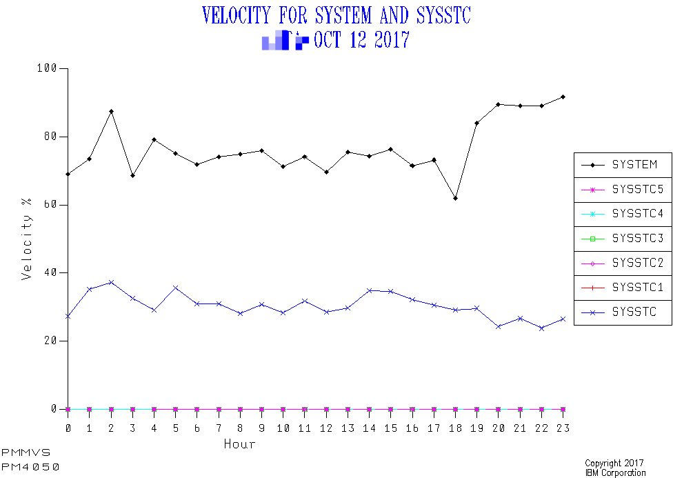
From the very same data set in that screencast I saw something I’d not noticed before: SYSSTC velocity is alarmingly low.

The above is one of four systems. Each has a persistently low velocity in the range 25% – 40%.

I didn’t expect this. To be honest, I’ve never looked at SYSSTC Velocity before. And what made me see it was adding the above graph to my kitbag a few months ago ¹ . (That and what happens to Importance 1, 2, etc Goal Attainment.)

Never having looked at SYSSTC velocity I have no real basis for an expectation, but this seems alarmingly low. And as I see more customer data I’ll form some “folklore in my head” 🙂 about it.

So this begs the question “what is it that is making SYSSTC’s velocity so low?” The search for an answer has to start with understanding which Delay component drags the velocity down. In this case it is Delay For CPU (and not zIIP, by the way).

I would’ve thought SYSSTC was relatively protected from CPU queuing ² but the data tells us otherwise. But consider two things:

• The low velocity is pretty consistent across the day.
• We know – from the previous blog post – there can be substantial CPU in SYSSTC at times.

So, it’s not really workload driven. So I suspect the LPAR set up and other things going on in the machine. A vague diagnosis for now. But at least I suspect something 🙂 – and that’s quite an advance.

Now why is this important? If you’ve reviewed Get WLM Set Up Right For DB2 you’ll know that key address spaces, such as DB2 / IMS lock managers (IRLM), run there. Without good access to CPU these address spaces will damage performance across a wide range of work.

So this is an unusual situation – until I keep seeing this in customers. 🙂 But it’s one worth looking out for.

One final thought: I probably should suppress the graph lines for SYSSTC1 – SYSSTC5 if there is no CPU in them. Oh to have some spare time. 🙂

(Originally posted 2017-11-05.)

For once this isn’t a blog post that discusses a podcast episode or a screencast. It is one where I feel a little exposed, but only a little.¹

I just updated my “Even More Fun With DDF” presentation – after a whole two months. You’d think there’d be little new to say after only two months, but you’d be wrong. Quite apart from some other additions, there is a whole new thought² to share. And I’m interested in opinions on it.

I think it’s a quite important thought: WLM Controls Are Not Enough For DDF.

Let me explain.

Traditional DDF Control Mechanisms

As you probably know, you classify DDF work below the DB2 address spaces and based on multiple potential qualifiers. Each transaction is a single commit³. Which is often just a small part of the requestor’s conversation with DB2. And WLM doesn’t know about the whole conversation, just the (independent enclave) transaction.

You can use period aging – so as a transaction accumulates service it can fall into periods 2, 3, and maybe 4⁴. You would expect each successive period to have a looser goal and a lower importance.

You can also use Resource Groups – but I consider that a pretty blunt instrument.

Where Does This Fall Short?

It falls short in two main areas:

• Non-Performance Controls
• Short Transactions

Non-Performance Controls

It might be stating the obvious but this is important: WLM does not control access to DB2.

So, you have to set up Security in DB2 and your security manager (such as RACF). You not only have to decide who can access a given DB2 and from where but also what they can do.

This is not a performance issue as such, but it’s the first clue that DB2 and Security people need to be involved in discussions about how to manage DDF work.

Short Transactions

A very short transaction is difficult to manage in any case. A bunch of all-the-same short transactions doubly so. There’s no period aging to be had there, for one.

This is the new area for me: I’m seeing in several recent cases bursts of short transactions from the same source. Two examples come to mind:

• SAP Batch. Which is really a bulk insertion of short DDF transactions.
• Java Batch. Likewise, quite often.

One thing these have in common is that they are generally⁵ detectable. The Unit Of Work ID⁶ is a constant for the “batch job”.

But this doesn’t really help control them. For that you really need gating mechanisms in DB2 / DDF and maybe outboard of that. And that’s really the new point.

To be fair, for SAP Batch, you generally see a Correlation ID of xyzBTCnnn where xyz is a kind of application code and nnn is a three-digit number. So you could classify it in a separate Service Class from e.g. SAP Dialog transactions (xyzDIAnnn).

Two Parting Thoughts

Another thing that occurred to me is this: Control of DDF is important not just for System purposes but to protect other DDF from rogue⁷ DDF.

Consider DB2 logical resources such as DBATs, which are a subsystem-level resource. If rogue DDF work came in and used them all at once it could crowd out Production DDF. And there’s plenty of that around that matters. So you definitely want to protect Production DDF. Probably with DDF Profiles, but with other DB2 mechanisms as available. And this is where I chicken out and defer to people like Rob Catterall – and posts such as this.

And one final thought: Slowing down DDF work might not be all that helpful, particularly if it holds locks that other work needs. But then this is true of other work, like lower-priority batch jobs. So WLM controls might have an unfortunate effect.

(Originally posted 2017-10-31.)

Hot on the heels of Screencast 11 – DDF Spikes is my latest screencast: Screencast 12 – Get WLM Set Up Right For DB2.

In it I talk about the important topic of ensuring DB2 is protected against shortages of CPU (and zIIP). There are a couple of quite nice examples to illustrate the point.

I should note that I don’t see instrumentation that explicitly shows what happens when IRLM gets heavy competition for CPU. I’m more concerned to show – as one of the examples does – that DBM1 can be significant so it’s worth keeping below IRLM.

Production Notes

This was the first time using Camtasia where I pruned out silence at the final – audio and video recombined – stage. I think I’m finally getting the hang of the tool and there’s a certain amount of muscle memory developed now.

Also, and I hope it doesn’t show too much, my editing of the audio (with Audacity) involved getting rid of a lot of huffing and puffing. I’d like to believe I wasn’t getting (too) old (to record) 🙂 and that this was just a cold. It seemed to me the more excited I got the less the huffing and puffing. I’m not sure if there’s a life lesson there or not. 🙂