(Originally posted 2017-10-30.)

It’s been a busy few weeks but we’ve a new episode out.

The experiment with narrowing the “stereoscape” was an interesting one. It is always going to be effort to do this, but having edited all 5 segments I got quite good at it. I think I maybe narrowed it a little too much, but I’d be interested in how it sounds to y’all. To my ears Marna and I (and indeed our guest and Marna) are coming at you from discernably different points, but it’s not too harsh.

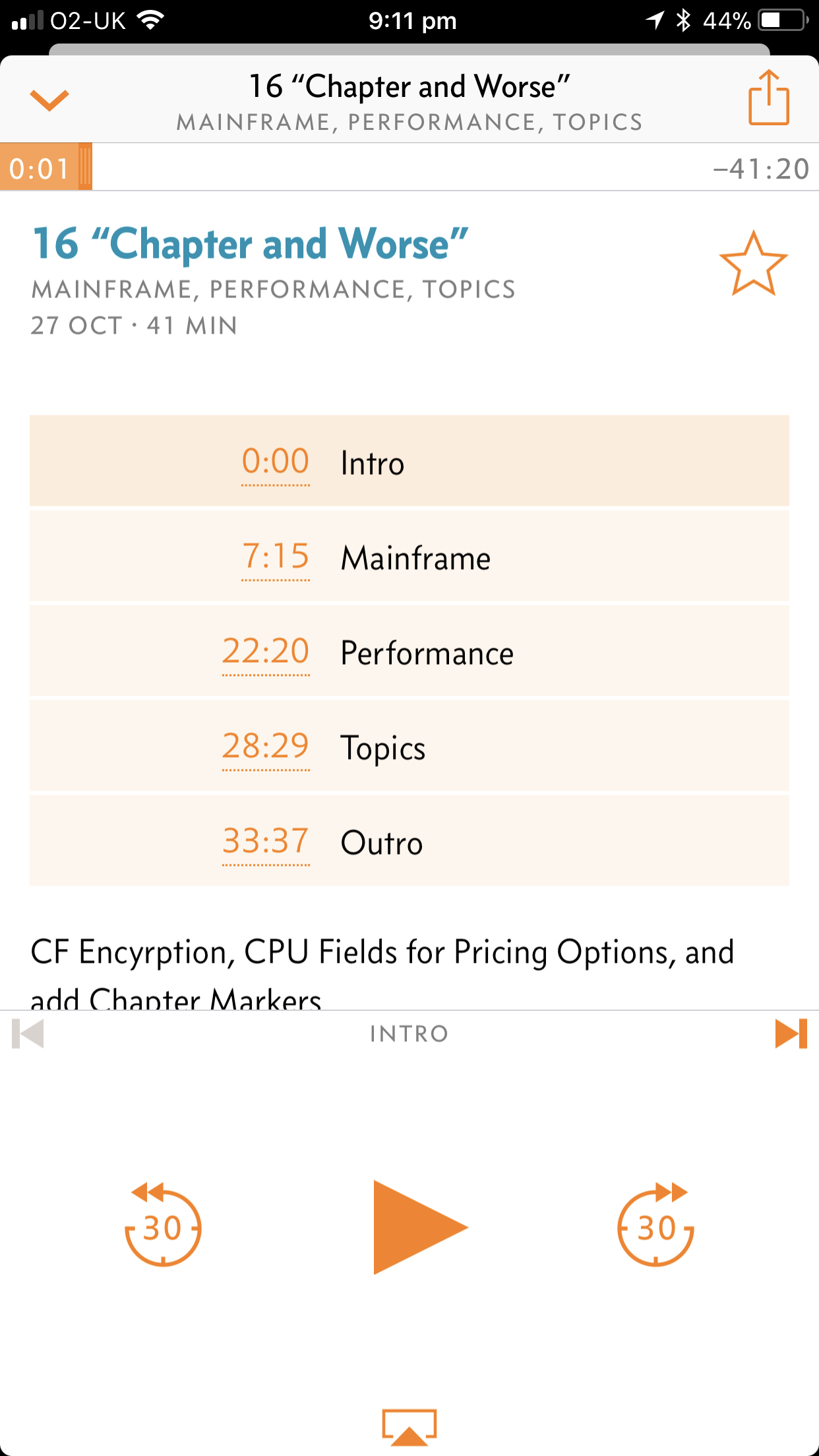
This is the second episode where I added chapter markers. In case you’re not able to see them in your podcast client this is how it looks on my phone:

Anyhow, we hope you enjoy this show. Here are the show notes.

Episode 16 “Chapter and Worse” Show Notes

Here are the show notes for Episode 16 “Chapter and Worse”. The show is called this because our Topics topic is about adding chapter markers (and pictures!) to our published MP3 file. We hope those of you that can see them enjoy them.

Where we’ve been

Marna has just returned from conferences and events in Johannesburg ZA, Chicago IL, and Munich Germany.

Martin has been to Munich Germany, and also visited a customer in Siena Italy.

Feedback

We have received feedback (in person, in Munich!) that our stereo separation of the channels was a little dizzying. Martin will be trying to make it less severe to relieve this effect.

Thanks for the feedback; We want to hear more!

Follow Up

Martin and Marna talked to the developers of the DocBuddy app, about their new release.

The latest release is 2.0.1, and has added a lot of social aspects (and fixed reported problems). The ability to look up messages is still there, but z/OS V2.3 isn’t there yet. We anticipate it will be coming soon, though, as it is important.

You can sign into the app (very easy to do!), and subscribe to Products and People, and discover them. People are “Influencers” and can be subscribed to. Products doesn’t include all the core z/OS elements, but Communications Server is there and has been active.

Feedback can be given, it’s an email under “Settings”, which took us a while to find.

Mainframe

Our “Mainframe” topic discusses a new z/OS V2.3 function, Coupling Facility Encryption, with Mark Brooks, Sysplex Design and Development. Mark talked about this latest capability in Sysplex, which has been getting a lot of attention as part of the larger Pervasive Encryption direction.

Mark explained that CF Encryption means that the customer’s data is encrypted by XCF in z/OS, sent along the link as encrypted, and stored as encrypted on the Coupling Facility.

z/OS sysprog needs to set it up by:

• using new keywords on CFRM policy on a structure by structure basis

• putting it in your CFRM couple data sets, and the policy change will be pending

• rebuild the struture (to get it from unencyrpted to encrypted)

• DISPLAY XCF structure commands can be used to see what the policy has, what the structure currently is, and the form of encryption used.

List and Cache structures contain customer sensitive data, the XCF control information will not be encrypted because it is not sensitive customer data. Lock structures don’t contain sensitive customer data, and are not encryptable.

Software requirements:

• z/OS V2.3. Strongly recommend not using CF encryption in production until fully at z/OS V2.3.

• ICSF. Need to have ICSF to generate keys and talk to the crypto cards. Every system in sysplex needs to be running with the same AES master key (meaning, same PKDS), note this requirement!

• XCF generates the key from ICSF services and stores that wrapped key inside the CFRM couple data set.

Hardware requirements:

• CPACF

• Encryption is performance sensitive, because it is extra work to encrypt and decrypt. You want it to be executed quickly. Encryption is host-based, and zEC12 has these facilities, however the older machines are not as fast as a z14. Take that into consideration.

Tooling:

• zBNA looks at new SMF data, so that you can see the amount of data transferred to the CF. From there, you could judge the cost of doing the encryption.

• SMF 74 Subtype 4 records contain the new information on the amount of data, via measurement APAR OA51879 on z/OS V2.2. Planning can begin on z/OS V2.2 with this APAR.

For more information, see the z/OS Setting Up a Sysplex.

Performance

Martin talked about MSU-related CPU fields for doing software pricing analysis. Some of these fields are used by SCRT in support of the new Mobile function.

Most notably the fields cover:

• Mobile Workload Pricing (MOBILE), using a new WLM mechanism, is available to many customers today. (The old way of doing Mobile Workload Pricing has been around for quite a long time.) Note a misrecording of IMS Mobile CPU at the Service Class Period level, which is fixed in IMS V15 APAR PI84889 and IMS V14 APAR PI84838.

• CATEGORYA and CATEGORYB: These are just placeholders for any future additional pricing options that come about.

These categories of CPU/MSUs are brought to life using the Workload Manager ISPF panels, using a new reporting attribute. You scroll twice to the right to get there. The values in the field can be MOBILE, CATEGORYA, or CATEGORYB.

Container Pricing is another pricing model, ….., and maybe another topic on that later.

The overall idea: Be aware of the new fields that you will be analysing. These fields are available at two levels:

• At the System level, as Rolling 4 Hour Average numbers – in SMF 70 Subtype 1.
• At the Service Class Period level, as interval-based numbers – in SMF 72 Subtype 3.

Topics

Our podcast “Topics” topic is about adding chapter markers to the MP3 file for podcast apps. This makes it nice to skip from one section to another easily. Our podcast has five sections, each with its own graphic and chapter.

Copyright on the MP3 specification expired finally in 2017, allowing more things to be done with the format. Chapters is one of them.

Martin adds the chapter markers into the MP3 file after doing the audio editing with Audacity. He then takes the MP3 file, and runs it into another tool on iOS called Ferrite. Audacity doesn’t have the ability to mark chapters (or to add the graphics), but Ferrite does. Hence it has to be processed with this second program to give the final MP3 chapters and graphics! (Ferrite was among the first tools to support Chapter Markers, with or without graphics.)

On Martin’s iOS podcast app, Overcast, he sees the chapter markers and graphics fine. Marna uses Android and CastBox, in which she cannot see them. She then tried another Android app, PodcastAddict, which claimed to have chapter support, and yet she still doesn’t see them. So it goes. 🙂

Customer Requirements

RFE 100505 Specify DSN HLQ for Healthchecker Debugging

The quoted description is: When the Healthchecker DEBUG option is turned on, the Healthcheck needs to write to a dataset. If that HLQ is not defined to security (in the case of Top Secret), the Healthcheck will fail. The customer then has to get this HLQ defined and appropriate access granted. I would like the customer to have the ability to control the DSN that the Healthcheck writes to.

Our discussion:

• Those checks which are added by the check writer themselves, usually during initialization with HZSADDCK service, set the HLQ. Right now, these checks are not changable by the user for DEBUG, which is what the requirement is all about.

• Sounds helpful, and desirable to have control of the high level qualifier(s) of the data sets. We agree.

• A likely solution would be to put it in HZSPRMxx, and allow the customer to control it (hopefully) across several checks.

Where We’ll Be

Martin will be in Whittlebury UK 7-8, November for GSE UK.

Marna will also be in Whittlebury UK 7-8, November for GSE UK with Martin. Then, at the big IBM Z event Systems Technical University in Washington, DC, 13-17 November. Then, in Milan, Italy 28-29 November for a System Z Symposium.

On The Blog

Martin published one blog post, which highlights a screencast of his:

• Screencast 11 – DDF Spikes

Marna has an idea for a blog, but needs more time to do some testing for it. It will be coming!

Contacting Us

You can reach Marna on Twitter as mwalle and by email.

You can reach Martin on Twitter as martinpacker and by email.

Or you can leave a comment below.

(Originally posted 2017-10-24.)

It’s been a month since I last did a screencast – and boy what a busy month I’ve had.

And in that month I had the privilege of working with a very nice customer, exercising my DDF Analysis code.¹

As so often happens, a graph or two come together to tell a nice story. One I shared with the customer, and one I’m sharing with you.

Because graphs are involved the natural medium for sharing it is a short video, so that’s what I made. You can find it here.

I think the background to the topic is quite important, so I preface the actual customer case with some educational material. Indeed there is a key point I’m keen to get across:

Guarding against ill-behaving (or “feral”, as I like to call it) is important. It’s insufficient to rely on Security mechanisms and DB2 controls to avoid feral DDF misbehaving. And misbehaviour matters. In the example I give it’s CPU – both GCP and zIIP – that is consumed by the engineful². But it might be precious DBATs, or other DB2 resources.

To clarify, while most people are interested in CPU as it relates to capacity planning (and software cost), I’m more worried about bursts of CPU affecting critical infrastructure. Though, I’ll admit, a (thick) veneer of “low value” DDF usage through a protracted period is worth managing down.

But this isn’t an easy phenomenon to control, particularly for egregious short-commit-scope work (aka bursts of small transactions).

One of the key sources of data is DB2 Accounting Trace (SMF 101) because it gives much finer timestamp granularity than RMF SMF. Further, the ability to identify a spiky consumer is pretty good. I advocate summarising at the 1-minute level, perhaps breaking out by IP address or Authid. This is realistic for me as I’ve built some nice DFSORT-based code to do the analysis.

The graphs come from CSV files created by this code. The question is whether you, dear reader, have access to a way of summarising individual 101 records in this way. I would assume, for example, MXG would allow you to. But I can say that the DFSORT code I use is very fast and very light.

Anyhow, I hope you enjoy the video (and the others in the series).

(Originally posted 2017-09-06.)

So this is a shorter episode, much to Marna’s pleasure. (Personally I’m indifferent to show length, regularly listening to episodes of other podcasts that run to 1.5 to 2 hours.)

It was very good to have a guest: Barry Lichtenstein. (I kept in the bit where I mispronounced his name, as I thought it a funny mistake[1]. You’ll find another piece of flubbing, again because it was funny.)

Enjoy!

Episode 15 “Waits And Measures” Show Notes

Here are the show notes for Episode 15 “Waits and Measures”. The show is called this because our Performance topic is about LPAR weights, and because this episode was after a seasonal hiatus.

Where we’ve been

Martin has been to nowhere in person, but has talked on the phone to several interesting locations.

Marna has just returned from SHARE in Providence, RI and from Melbourne, Australia for conferences.

Mainframe

Our “Mainframe” topic discusses a small new function in z/OS UNIX that there were customer requirements for, and that might not have been highlighted as much as other new functions in z/OS V2.3: automatic unmount of the version “root” file system in a shared file system environment. Our guest was Barry Lichtenstein, the developer of the function, and he told us all about it:

• there is a new BPXPRMxx VERSION statement parameter, UNMOUNT. This means that when no one is using that “version file system” (the new name for the “version root file system”!), it will be automatically unmounted. This is not the default. Syntax here
• this function is nice, as it will allow an unused version file system to be “rolled off” when you don’t need it anymore. Unused here, means that no system is using it or using any file system mounted under it. z/OS UNIX will do this detection automatically, and unmount not just the version file system, but mounted file systems under it that are no longer used by any systems after an unspecified amount of time.
• you can turn this on and off dynamically with a SET OMVS or SETOMVS command. There is DISPLAY command support of it. And perhaps the best news, the health check USS_PARMLIB will see if the current settings don’t match the used parmlib specification. (Marna thinks this check is the gold standard for using dynamic commands and not regressing them on the next IPL with the hardened parmlib member!)
• we weren’t sure if SMF record 92 would be cut when the unmount happened, but Barry said nothing unique was happening for this function so what happens today is most likely the same behavior. There are messages that are issued in the hardcopy log when the unmounts happen. SMF 90 might be issued for SET changes.

Performance

Martin talked about Weights and Online Engines in LPARs, and Martin again looking at customer information.

• Intelligent Resource Director (IRD) changed PR/SM worked:
  1. Dynamic weight adjustment
  2. Online logical engine management (vary online and offline). Shows minimum and maximum weights when changed by IRD.
• HiperDispatch: took away logical engine management (and manages it better!), and kept IRD dynamic weight adjustment. With HiperDispatch’s parking of engines, no work is directed towards it. An affinity node is a small group of logical engines to which a subset of the LPAR’s work is directed.
• More instrumentation was introduced, such as Parked Time and refined instrumentation on weights (vertical weights, by engine).
• Customer situation was that they did their own version of IRD and HiperDispatch: Varying logical engines online and varying weights (not using IRD itself). Martin expected IRD to change weights, but he saw the IRD weight fields were all zero. You must look at the “inital weights”, which means initial since you last changed it.
• Why not let IRD do it? Martin thinks there was something in the customer’s mind to control it themselves, perhaps somethind other than WLM goal attainment (which IRD would adjust weights for).
• Why not use HiperDispatch? Martin thinks that maybe a subtle difference might be needed, but LPARs should be designed properly. One possible aim might be to fit in one drawer, for instance. Maybe it’s not understanding what HiperDispatch does.
• How did the customer adjust the weights? It was an open question. Probably via BCPii? Feedback would be welcome on this.
• As an aside, with IRD a change in weights would lead to HiperDispatch recalculating how many Vertical High, Medium, and Low logical engines each LPAR has.

Lesson learned: Assumption on how something has dynamically changed may not always be correct.

Topics

Our podcast “Topics” topic was “Video Killed the Radio Star?” and about screencasting.

Martin has been trying to post screencasts to YouTube. Here’s one.

Screencasts are not videos where you see the speaker. It’s just a visual of what is happening on a screen with a talkover.

The best candidates are graphs and program output. Martin uses these steps to create these screencasts:

1. First, make a set of slides or images. Annotations are good to use, to point to a particular feature on the screen. (They don’t have to be animated.)

2. Use the screen recorder to add sound to the slide. (In PowerPoint, record the slides.)

3. Editing, with proper fadeouts. Split the audio out and clean it up with Audacity.

4. Re-unite the audio and the video. Camtasia, while expensive, has some promise.

5. Publish on Youtube.

Customer Requirements

As well as Barry’s mention on the v/OS V2.3 automatic unmount of version file system requirement (RFE Number 47549, “Automatic disposal of z/OS UNIX version root”), there was another customer requirement we discussed:

RFE 97101 Make /dev/random available on z/OS without ICSF dependency

The quoted description is:

/dev/random is a special file that serves as a psuedo-random number generator source for applications. On z/OS, this special file is only provided if ICSF is started. If ICSF is not available, we need to resort to some other source of random numbers (which will have to be implemented within applications). Goal here is to make /dev/random available on z/OS, independently of whether ICSF is available or not.

Our discussion:

• It’s a major migration action in z/OS V2.3 to have ICSF available for /dev/random.
• ICSF is a dependency for many functions. It’s important to have on every single z/OS system.
• Another aspect: each user had to have authority to use these ICSF services for certain of the functional depedencies (including /dev/random).

Martin mentioned that random number generators vary in quality, and behaviour. He hopes, if this were done, it would be high quality. One criterion would mean a close enough match to the ICSF-based algorithm, distributionwise.

Where We’ll Be

Martin will be in middle of Italy in August, 2017. He is threatening to drive from Italy to the Munich zTechU conference.

Marna will also be in Munich too. Marna is going to Johannesburg for the IBM Systems Symposium, aka IBM TechU Comes to You. She is also going to Chicagoland area on Sept 26 and 27, 2017 for some area briefings.

Both Martin and Marna are hoping to do a poster session in Munich, which should be jolly good fun.

On The Blog

Martin has actually not published a blog recently!

Marna actually did publish a blog recently!

• Some handy z/OS V2.3 and z14 information

Contacting Us

You can reach Marna on Twitter as mwalle and by email.

You can reach Martin on Twitter as martinpacker and by email.

Or you can leave a comment below.

(Originally posted 2017-07-14.)

If a customer has Transaction goals[1] – for CICS or IMS – it’s possible to observe the CPU per transaction with RMF.

But you have to have:

• Transaction rate
• CPU consumed on behalf of the transactions.

This might seem like stating the obvious but it’s worth thinking about: The transaction rate and the CPU consumption have to be for the same work.

Now, a Transaction service class doesn’t have a CPU number. Similarly, a Region service class doesn’t have transaction endings.

So you have to marry up a pair of service classes:

• A Transaction service class for the transaction rate.
• A Region service class for the CPU.

Operationally this might not be what you want to do. Fortunately, you can do this with a pair of report classes.

There’s another advantage to using report classes: You can probably achieve better granularity – as you can have many more report classes than service classes[2].

So I wrote some code that would only work if the above conditions were met[3].

Unimaginitively my analysis code is called RTRAN; You feed it sets of Transaction and Region class names.

Perhaps I should’ve said you could have e.g. a pair of Transaction report classes and a single Region report class and the arithmetic would still work[4].

But why do we care about CPU per Transaction?

There are two reasons I can think of:

• Capacity Planning – by extrapolation
• Understanding what influences the CPU cost of a transaction

From the title of this post you can tell I think the latter is more interesting. So let’s concentrate on this one.

In what follows I used RTRAN To create CSV files to feed into spreadsheets and graphs[5]. Over the course of a week I captured four hills while developing RTRAN.

The first thing to note is that CPU per Transaction is not constant, even for the same mix of transactions.

This might be a surprise but it makes sense, if you think about it. But let’s think about why this could be.

Two Important Asides

But first a couple of asides on this method:

• Take the example of a CICS transaction calling DB2. While most of the work in DB2 is charged back to CICS not all is: There is a significant amount of CPU not charged back[6]. It’s highly likely the DB2 subsystem is shared between CICS and other workloads, such as DDF and Batch; It gets much less satisfactory trying to apportion the DB2 cost so I simply don’t.

• Likewise, I’m ignoring capture ratio. While it would be wrong to believe it’s constant, for most of customers’ operating range it’s a fair assumption to go with a constant value for capture ratio.

In a nutshell, both these asides amount to “this is not a method to accurately measure the cost of a transaction but rather to do useful work in understanding its variability.”

Why CPU Per Transaction Might Vary

I’m going to divide this neatly in two:

• Short-Term Dynamics
• Long-Term Change

Short Term Dynamics

CPU per transaction can, demonstrably vary with load. There are a couple of reasons, actually probably more. But let’s go with just two:

• Cache effects, that is more virtual and real storage competing for the same scarce cache.
• If a server becomes heavily loaded it might well do more work to manage the work.

But it’s not just homogenous variation; Batch can impact CICS, for example.

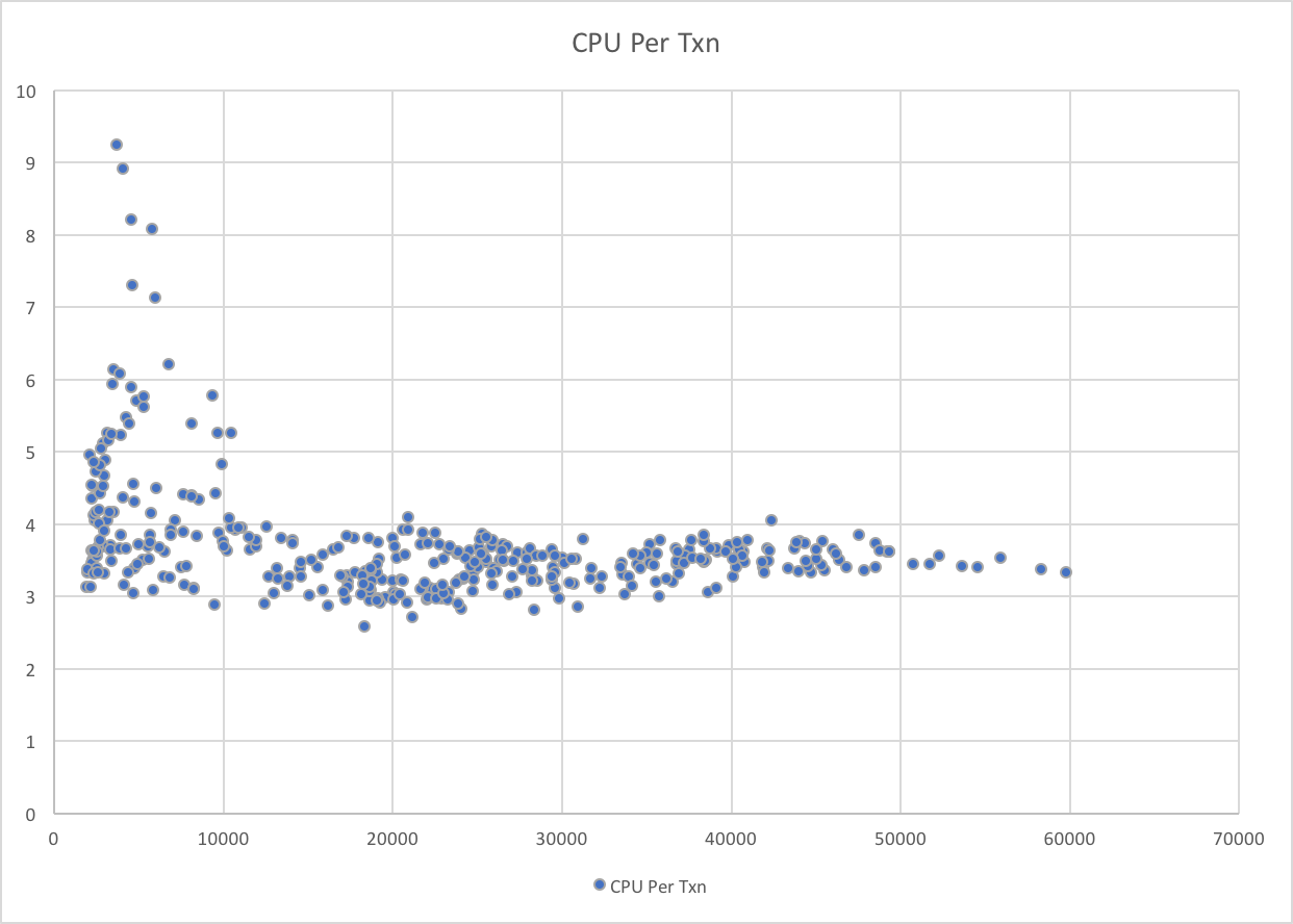
Look at the following graph:

In this case it’s the lower transaction rates that are associated with the higher CPU per transaction. But not all low transaction rate data points show high CPU per transaction.

A tiny bit more analysis shows that the outliers are when Production Batch is at its heaviest, competing for processor cache. It’s also the case that these data points are at very high machine utilisation levels, so the “working more to manage the heavy workload” phenomenon might also be in play.

Long Term Change

“The past is a foreign country; they do things differently there” L. P. Hartley The Go-Between.

Well, things do change, and sometimes it’s a noticeable step change, like the introduction of a new version of an application, where the path length might well increase. Or, perhaps, a new release of Middleware[7]. Or, just maybe, because the processor was upgraded[8].

But often, perhaps imperceptibly, CPU per transaction deteriorates. For example, as data gets more disorganised.

Conclusion

If it’s possible to do, there’s real value in understanding the dynamics of how the CPU per transaction number behaves.

Try to understand “normal” as well as behavioural dynamics, and watch for changes.

(Originally posted 2017-07-08.)

I’m writing this under a lovely cherry tree in my back garden, in cool shade on a warm summer’s day. Before you complain “that ain’t working” I’ll just point out this is on a Saturday afternoon. 🙂 And the “air cooling” is what makes this post possible. 🙂

Just this past week I began an experiment. As with all experiments I might continue with it, but I might not; It depends on whether people find it interesting or valuable.

One of the nicest things about my job is when a truly interesting graph or diagram appears in front of me, especially if it’s the result of some programming of mine. This week has been full of such moments, as I’ve developed some new code. (More of that in a different post, I think.)

And the week started with an episode of Mac Power Users talking about screencasting.¹

About 10 minutes into the episode I suddenly thought “I could use screencasting to talk about some interesting graphs”. For once, I had the discipline to listen to the rest of the episode before doing something about it. I will admit I was fair chomping at the bit. 🙂

My development approach this week has been the nearest to disciplined I think I’ve ever been. 🙂 It turns out I had four hills to capture. Because I might have to stop with only a few hours’ notice this is a nice characteristic. Each hill took about a day and I promoted into Production after each hill was captured.

Agile? More like Fragile. 🙂

And so after capturing the first hill I recorded my first screencast:

• Screencast 0 – CICS CPU Per Transaction

This was pretty basic; I’m just moving the pointer around on a single graph while I talk.

After the second hill I recorded my second:

• Screencast 1 – CICS CPU Per Transaction, More Of The Story

This time I had three graphs to show, building on the story from Screencast 0.

But then I thought I would take one of my “in Production” graphs and annotate it. It’s one that has nothing to do with the first two but one I very commonly use:

• Screencast 2 – DB2 Data Sharing LOCK1 Structure Dynamics

Here I used Pixelmator for Mac, which is rather overkill. I take the base graphic (a PNG) and create more graphics with successive annotations. It actually was unwieldy, given I don’t have much experience with Pixelmator.

Then I captured a third hill, which led to:

• Screencast 3 – CPU Per CICS Transaction As The Machine Gets Busier

This time I used the much simpler (and built in to Mac OS) Preview to annotate. It did indeed take much less time, though it would be fair to note it’s only a single “base” slide.

And finally, for now, it was really quick to illustrate the capturing of the fourth hill with:

• Screencast 4 – CICS Transaction Statistics Across Multiple Systems

At this point point I realized my screencasting might be a “thing” so then the question of “materials management” came up. My answer is just to shove each screencast (episode) in its own folder. I feel vaguely organized now. 🙂

Thoughts

It’s occurred to me this is quite a light-weight teaching aid. So when I develop new code I might well use this to explain the value, issues and nuances.

It also occurs to me that anyone – certainly on a Mac – could produce (and share or publish) material like this. And if you had, say, presentation slides to give you might do it this way.

As you can see, I’m experimenting with annotation tools. So far I’ve used two on the Mac – preparing them as static graphics before recording. I also have several on iOS, most notably Pixelmator for iOS and Annotable. What I’m not doing is annotating the video itself. I probably should get round to audio clean up and video editing; I’m not sure how I’ll do that. ²

One stance I deliberately took was to produce short but frequent videos. I think that makes it less daunting to do and possibly more consumable for the viewer.

I don’t know if I’ll commit to keeping on going. Certainly daily (my current rate) seems too aggressive and weekly too infrequent. That depends on the viewership. I certainly think material is going to keep appearing that this medium would be well suited to.

Nobody would call me “camera shy”. 🙂 But the effort of recording and editing pieces to camera seems to me quite high, with little value. This, however is much easier to do. So I don’t think I’m going to do videos with me in them – unless something changes my mind.

This is – to me – a great toe in the water. I hope it is to you, too.

(Originally posted 2017-07-07.)

Boy has this one been a “slow train coming” but I’m glad it’s out now. And it was fun making it. Especially the piece with Frank and Jeff.

It’s a long listen; As always I’m comfortable with long podcast episodes.

Enjoy!

Episode 14 “In The Long Run” Show Notes

Here are the show notes for Episode 14 “In the Long Run”. The show is called this because the episode ran longer than usual, and it is of fitting length if you have a very long commute.

Follow-ups

Martin has two new blog posts about DDF (DB2’s Distributed Data Facility), following up on Episode 13 where he talked about recent DDF analysis enhancements:

• A Tale Of Two Batteries

• Happy Days Are Here Again?

(Follow Up is of course an invention of John Siracusa.) 🙂

Where we’ve been

Martin has been to London (to the UK GSE zCMPA User Group) to present his ever-updated DDF presentation, and had more fun with it.

Marna has been to the Systems University in Orlando, Florida (May 22, 2017 week).

Mainframe

Our “Mainframe” topic is the first in a series of deep dives into z/OS V2.3. Part 1 is on z/OSMF Autostart.

This is the most important migration action in z/OS V2.3, and requires special consideration by every customer IPLing z/OS V2.3. Things that you’ll need to consider are:

• Whether to start z/OSMF or not. (Starting is the default). You control this via IZUPRMxx parmlib members (which in new news can be shared via PI82068).

• If you don’t start z/OSMF and have its functions available to system(s), then you not be able to use certain functions (notably in z/OS V2.3: JES3 Notification).

• If you don’t want to start z/OSMF on a certain system, you can connect to another z/OSMF system in the same sysplex, and that requires specification on which group that would be.

• The number of z/OSMF servers in a sysplex hasn’t changed, still as it was before V2.3.

• z/OSMF server starting on an LPAR with good zIIP capacity, and memory (minimum of 4GB) is a starting consideration.

• Strong recommendation: start z/OSMF now on your V2.1 or V2.2 system so that there are fewer work items to do (a couple of security profiles, new procs, parmlib updates only).

Performance

In our “Performance” topic Martin talked about two Parallel Sysplex items that he’s been pondering extensively recently. He’s been using RMF data (taken from SMF type 74 subtype 2 and 4).

Coupling Facility

This is the subject of a blog post: Some Parallel Sysplex Questions, Part 1 – Coupling Facility

• Resources: CPU, memory, and path

• Structures: their role to applications, and how responsiveness responds to work load is interesting

XCF Signalling

This is the subject of another blog post: Some Parallel Sysplex Questions, Part 2 – XCF

• Resources: Paths, buffers, and transport groups

• Groups: again, knowing the application types, with the theme of managing traffic down when possible

Topics

Our “Topics” topic is subtitled “Podcast meets Podcast” with the newest mainframe podcast we know: Terminal Talk.

Frank De Gilio and Jeff Bisti are the hosts, and concentrate on a wider introductory perspective than our MPT podcast does.

• Terminal Talk (TT) has enviable technology for recording, and came about from Frank and Jeff taking long car rides to Pennsylvania.

• Planning for the TT podcast consists mostly on engaging guests, and not necessarily following an outline.

• Length is a big consideration: TT is intended to be of a work-commute length.

• Editing is done with Audacity, just like our MPT podcast. TT records mono. MPT does stereo. Martin uses the Audacity waveform visualisation when editing; Hence the terms “um fish” and “so so birds”. 🙂

We had great fun talking to Frank and Jeff; Martin left some of the laughs in the final edit. And we’re sure a lot of you will enjoy Terminal Talk, having listened to all their episodes so far.

Customer Requirements

Marna and Martin discussed three customer requirements:

• DSS needs to support Extended TIOT

• Update of an OpenSSH

• Option to suppress override messages from SMFLIMxx on z/OS 2.2

<–! * 76875 and 75766: Migration check for CF structure sizes “at risk” due to impending new levels of CFCC –>

Where We’ll Be

Marna will be at SHARE in Providence, RI, 7–11 August 2017 and [IBM Systems Symposium, 15–17 August 2017 in Melbourne, AU)[https://www.regonline.co.uk/registration/Checkin.aspx?EventID=1939263]

Martin will be going nowhere for a while.

On The Blog

Martin has published six blog posts recently. The two not already mentioned are:

• Give Me All Your Logging
• Some Lessons On DFSORT Join

Marna has not blogged since our last podcast episode.

Contacting Us

You can reach Marna on Twitter as mwalle and by email.

You can reach Martin on Twitter as martinpacker and by email.

Or you can leave a comment below.

(Originally posted 2017-06-25.)

Back in 2009 I wrote about Performance of the (then new) DFSORT JOIN function.

This post is just a few notes on things that might make life easier when developing a JOIN application. Specifically the one I alluded to in Happy Days Are Here Again? when I talked about processing SMF 101 (DB2 Accounting Trace) records.

And I wrote it having scratched my head for a few hours developing a JOIN application that will soon be part of our Production code.

Lesson One: Massage The Input Files In Separate Steps

This flies in the face of what I said in 2009 but bear with me. That post was about Performance in Production. Here I’m talking about Development, specifically prototyping.

Here is what “Single Step” looks like:

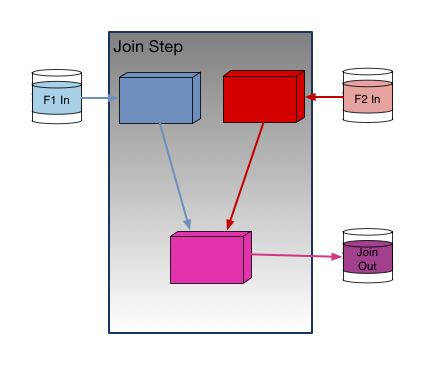
And this is what “Multiple Step” looks like:

The clear advantages of “Single Step” are:

• There is no need for intermediate disk storage (and I/O).
• It is simpler.

But sometimes you really want to know what the intermediate records look like. In particular what positions fields end up in, what lengths they have, and what formats they appear in.

And you can always move the logic to the JOIN step as you approach Production; In fact you should. SYSIN becomes JNF1CNTL for file F1 and JNF2CNTL for file F2.

Viewing Intermediate Files While Running JOIN

While you could run these pre-processing steps and stop before the JOIN step that isn’t actually necessary. You can still see the intermediate files if you could something like

OUTFIL FNAMES=(SORTOUT,TESTOUT)

and route TESTOUT DD to SYSOUT (or wherever). The SORTOUT data set can then be fed – as you originally intended – into the JOIN step.

In my case the two data sets fed into the JOIN are temporary; When the job completes they’re gone.

Lesson Two: Debug Failed Joins One Field At A Time

When I was developing my JOIN I had two unexpected (and wrong) things happening:

1. I got zero records out.
2. I got far more records than expected out.

Zero Records Out

This is the case where there were no matching records, or so it seemed.

In my application I’m joining on multiple key fields – 8 in my case.

Having got very confused for a while[1], I took the following approach:[2]

1. Try matching on one field.
2. If that doesn’t work, p out why. And fix.
3. Repeat with that field and another.
4. And so on.

By the way it’s probably best not to direct the output to the SPOOL; While I was debugging this way I was sending several million lines there before I caught and purged the job.

Far More Records Than Expected Out

This one was a little more difficult to debug. The net of it is the JOIN key – all umpteen fields of it – isn’t long enough (specific enough).

In my case I was using the first 22 bytes of the 24-byte Logical Unit Of Work ID (LUWID). And I was getting orders of magnitude more records out than I expected.

The final two bytes are a commit number. For some reason I thought it shouldn’t be part of the join key. I was wrong.

Extending the key to 24 bytes made the JOIN (demonstrably) behave.

Lesson Three: Careful With The Name Spaces

DFSORT doesn’t really afford multiple name spaces, so you have to fake them.

So for the F1 file you might prefix the symbols with “F1_” and, similarly, the symbols for the F2 file might begin with “F2_”.

Conventionally, I use “_” before the symbols that map a record after INREC. You could adapt that so the results of REFORMAT could be mapped using symbols prefixed with “_”.

In any case some sort of symbol scheme is needed.

While we’re talking about symbols, I wouldn’t attempt JOIN without them.

If you’re developing with the “Multiple Step” approach you can reuse the symbols between the reformatting and JOIN steps – because you can concatenate SYMNAMES data sets. But note this reusing the output symbols from the reformatting steps for the input to the join.

One thing you can’t do is specify different SYMNAMES DDs for the pre-processing stages in the “Single Step” case. So you have to be careful with names.

In case the above is clear as mud let me try a little example.

In F1 Step you might code:

//SYMNAMES DD DISPLAY=SHR,DSN=HLQ.F1.INPUT.MAPPING
//         DD *
POSITION,1
F1_A,*,16,CH
F1_B,*,8,BI
/*

And for the F2 Step you might code:

//SYMNAMES DD DISPLAY=SHR,DSN=HLQ.F1.INPUT.MAPPING
//         DD *
POSITION,1
F2_A,*,16,CH
F2_C,*,4,BI
/*

In the JOIN Step you might code:

//SYMNAMES DD DISPLAY=SHR,DSN=HLQ.F1.INPUT.MAPPING
//SYMNAMES DD *
* FROM F1
POSITION,1
F1_A,*,16,CH
F1_B,*,8,BI
*
* FROM F2
POSITION,1
F2_A,*,16,CH
F2_C,*,4,BI
*
* REFORMAT OUTPUT
POSITION,1
FLAG,*,1,CH
_A,*,16,CH
_B,*,8,CH
_C,*,4,BI
* OUTREC OUTPUT
__A,*,16,CH
... 
/*

Of course, in the above you’d probably put the F1_ and F2_ fields in their own symbols files – to enable reuse.

One minor annoyance with symbols files is they push you towards another ISPF session, which you could probably do without. But it is only a minor annoyance.

Lesson Four: REFORMAT Isn’t The Final Reformatting

I expected REFORMAT – which pulls the fields together from the two input streams – to allow formatting such as character strings.

It doesn’t. So you have to add them in an OUTREC or OUTFIL statement. A cumbersome alternative is to pass the fixed strings in as fields from the F1 or F2 streams.

One thing that is available in REFORMAT (and only from REFORMAT) Is a single-character indicator of how the record was matched. It has three potential values:

• 1 – only from F1.
• 2 – only from F2.
• B – from both F1 and F2.

This might prove useful In debugging. You indicate you want this flag using the “?” character.

Conclusion

So, these are the learning points from my second DFSORT JOIN application. If this looks complex I think it reflects some of the powerful complexity of DFSORT JOIN. I also think it’s fair to say complex DFSORT applications can be fiddly.

The one overarching thing in my mind is to build any DFSORT application up in simple stages, and perform optimisations later. A good example, which I’ve already shown you, is the “Multi Step” approach to building up JOIN.

(Originally posted 2017-06-20.)

I’ve written a lot about DDF and SMF 101 (Accounting Trace) over the years. It turns out my code went backwards a few years ago, and with good reason.

Let me explain.

But before I do, recall “my code” refers to a DFSORT E15 exit that “flattens” SMF 101 records, extracting the DDF-related fields into fixed positions. Each input record leads to an output record (if it qualifies). Downstream code does summarization but, crucially, records aren’t joined together.[1]

Happy Days

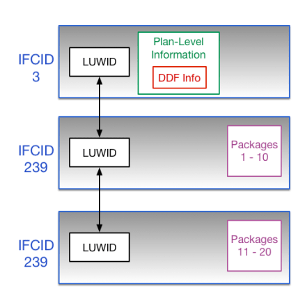
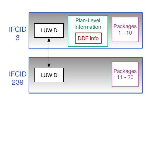
Prior to DB2 Version 8 package-level information was recorded in the main (IFCID 3) 101 record. IFCID 239 (also 101) records contained overflow package sections only, as shown in the following diagram. My code picked up the first few packages in the IFCID 3 record.

Notice the first 10 packages were in the IFCID 3 record, with the first IFCID 239 record containing up to 10 more, and so on.

The importance of package-level information for DDF is threefold:

• The initial package says a lot about the calling (usually distributed) application.
• Quite a lot of DDF applications work by calling Stored Procedures and User-Defined Functions (UDFs). We see that fine structure in the package-level information.
• You can, as usual, see where the time and CPU is being spent – to the package level.

Generally I could do my work without needing IFCID 239 records as the first 10 packages were described in the IFCID 3 record.

Life was goodish. [2]

Not So Happy Days

But then Version 8 came along and the structure of SMF 101 changed.

Now the IFCID 3 records don’t contain package information. All this is in IFCID 239 records now. So I couldn’t get information about the first two, say, packages for a DDF invocation. The colour drained out of this. 😦

I wanted, for example, to know which machines access IBM Content Manager and which functions they used. I probably see something mnemonic at the plan level in the IFCID 3 record. I definitely see something mnemonic in the IFCID 3 record but now they’re separate records. Never the twain shall meet.

So, reluctantly, I ripped the package analysis stuff out of my code. A good few years ago. And I was miserable. 🙂

And you’ve seen all the things I’ve been able to do with DDF with SMF 101s – in previous blog posts.

Happy Days Are Here Again

But then along came DFSORT JOIN which allows pairs of records to be efficiently joined together.

This is great but what would the key to join on be? It couldn’t be the time stamp – as the IFCID 3 and IFCID 239 records’ timestamps would usually be slightly different – and probably no combination of other SMF 101 record fields either. Well, some bits for the IFCID 3 and 239 records are common. In particular the Standard Header (mapped by DSNDQWHS). One field in particular stands out: The Logical Unit Of Work ID (LUWID).

As you can see in each of the diagrams the LUWID[3] ties the related records together.

So then there was hope.

So I extended my DFSORT E15 exit to emit two types of flattened record and the DFSORT invocation itself to write to an additional destination: DD IFCID239. So IFCID–3-originated records are formatted differently and go to different data sets than IFCID–239-originated records.

Now I can use join – very much in the style of Lost For Words With DDF. In that post I talked about joining Client and Server 101 (IFCID 3) records based on most of the LUWID. In this new case I can do something pretty similar.

At this stage I have thrown into production this code to write the flat files, having run some test reporting to verify my code works.

In my first set of data I see (as I mentioned above) IBM Content Manager callers, complete with nested stored procedures. I can tell they’re stored procedures because they have the appropriate flag set in the right sections.

Now to build some reporting based on these files and JOIN. Actually I can see some value in reporting on the IFCID 239 data alone.

Stay tuned for another thrilling installment. 🙂 Seriously, I fully expect to learn stuff, including some new tricks, as build on this foundation.

And as I finish this post off, sitting in my back garden 🙂 , I’ve jotted down a few notes on using DFSORT JOIN. So expect to hear more about that soon.

(Originally posted 2017-06-17.)

This post follows on from Some Parallel Sysplex Questions, Part 1 – Coupling Facility. Again it’s a high level treatment.

In contrast to Coupling Facility (CF), there is really only one type of resource: Signaling paths. But again application componentry is what brings it all to life. In this case it’s XCF groups and members.

And the motivation for all this? Responsiveness and (CPU) efficiency.

Most of what I do with XCF relies on the SMF Type 74 Subtype 2 record – which is dedicated to XCF.[1]

Signaling Paths

There are two kinds of signaling path:

• Channel To Channel (CTCs), using dedicated channels and cabling
• Coupling Facility (CF) structures, using the whole CF infrastructure

Signaling paths are owned by Transport Classes (TCs). In my experience most customers rely on transport classes shared between all XCF groups. Just occasionally I see TCs dedicated to specific groups. I’ve not seen a real case for this and would observe that a TC owns its own links so that might be the motivation. Fairly obviously that constrains XCF’s choices in which paths to send a particular set of messages.

Paths, of course, are between pairs of systems. Even if we’re talking about CF structure paths.

TC’s have their own set of output buffers in each system. These buffers have a specific size – controlled by CLASSLEN. You also define how many there are. Statistics in SMF 74–2 speak of Small Messages, Fit Messages, Large Messages (some With Overhead). There will be times when these statistics really matter, but these are few and far between.

“Small”, “Fit” and “Large” are relative to CLASSLEN – for the TC. Messages that are “Small” could’ve used a smaller CLASSLEN. This implies a (small) waste of memory. “Large” means a larger buffer had to be used. “With Overhead” is where this could really matter.

If you get the impression I don’t think Transport Class (TC) tuning is a major event you’d be right. It would be nice to have better message size statistics – such as distributions to enable a more scientific TC design, particularly of CLASSLEN.

One thing well worth doing is understanding which signaling paths are predominantly being used by their owning TC. In particular whether the traffic is refusing to use CF structures.[2]. I’ve seen cases – generally where the CF has shared engines – where all the traffic has gone via the CTC’s.

Groups And Members

As I said, groups and members are where the real fun is. Here are some reasons why:

• Among the heaviest CF structures are the XCF signaling structures
• Part of DB2 Data Sharing tuning is minimising LOCK1-related XCF traffic
• It’s interesting to see – at the address space level – who talks to whom. A good example of this is CICS regions talking, using the DFHIR000 XCF group[3].

74–2 reports members and groups, but not which Transport Class each group uses. So there isn’t a direct link between XCF applications and resources.[4]

For each member of a XCF group, you get traffic to each system. You do not get member-to-member traffic. So it isn’t possible to directly see who talks to who. And the “inference game” is somewhat fraught. As was pointed out to me, it’s not feasible to document a 2048 x 2048 sparse matrix in SMF 74–2.

Conclusion

Some of my comments above might lead you to believe all is not well with XCF instrumentation. I have to say the gaps are very minor, and more to do with nosiness than real performance work.

In terms of priorities for tuning Parallel Sysplex, XCF is the junior partner. But it is well worth examining, alongside Coupling Facility.

By the way, one of the things causing me to write these two posts was fixing a number of bugs[5] in my code which made me examine how we do Parallel Sysplex tuning. One in particular was that some of my code doesn’t translate from System Name to SMFID. My latest client has completely different System Names and SMFIDs.

(Originally posted 2017-06-15.)

In Some WLM Questions I outlined my approach to looking at WLM implementations. It was necessarily very high level, but the intention was twofold:

• To prime customers about the kinds of questions I might be discussing with them – if I ever saw their data.[1]
• To give anyone maintaining a WLM policy some structure. It remains my view that WLM needs care and feeding, on a not-infrequent basis.

You could argue these two purposes are essentially what this blog is all about.

So, this post does the same thing but for Parallel Sysplex. Actually it’s Part 1 of 2, dealing with Coupling Facility (CF) questions. The other part (covering XCF) will be along presently.

Again, expect a high level treatment. There are plenty of posts in this blog that talk at a more detailed level.

(Perhaps Superfluous) Disclaimer: This isn’t all about performance and capacity, because I’m not either.

I’ll structure this post in two pieces:

• Resources
• Structures

That’s how I look at Coupling Facility, so it seems as good a structure for this post as any.[2]

Note: Everything I’m talking about is instrumented with SMF Type 74 Subtype 4.[3]

Resources

If we were examining z/OS systems we’d start by looking at resources, so it’s natural to look at coupling facilities the same way.

The difference, though, is in what those resources are and how they behave. For example:

• Coupling facilities don’t do I/O in the conventional sense.
• Coupling facilities don’t page.
• Memory management is more or less static.
• Access to resources is not policy-driven; There is no WLM or SRM for coupling facilities.

So let’s examine the different types of resources.

CPU

In this piece I assume the coupling facility has dedicated processors.[4]

A basic metric is CPU utilisation. We talk a lot about how busy a coupling facility should be, both for steady state and for recovery situations. As a rough guideline, a CF that tops 40% is one where I would be concerned about the effects of growth. One above 50% I’d be more immediately concerned about. Here I’m touching on the topic of “white space”.[5]

Usually a sysplex has more than one coupling facility. While I wouldn’t be fetishistic about it, I would investigate the reasons for any significant imbalance.

Which brings us onto a point that strays into the second part of this post: We can readily see which CF structures drive CPU utilisation. So we know which structures might contribute to imbalance. We’ll come back to CF structure-level CPU in a bit.

Memory

Memory usage is much more static than with z/OS; You allocate structures and rarely change their size. But this doesn’t make CF memory a boring topic.

As with CPU, the memory instrumentation is good; You can, for instance, readily see how much is installed and how much is free. Again, the concept of “white space” exists for memory. Here, we’re more interested in recovering structures from a failing CF into a surviving one.[5]

But most of my discussions with customers about CF memory haven’t been about leaving space. I’m finding quite a few who have tons of free memory; The point has been to encourage them to exploit the memory. The structures discussion below touches on this also.

Talking of structures, my code calculates how much extra memory would be taken (and how much less would be free) if all structures went to their maximum size. Usually there’s plenty free, even if they did.

Links And Paths

In my experience link and path utilisation are rarely a problem, but there’s plenty of CF-level instrumentation for the cases where this is a problem. My guess is customers generally get this right. In any case the remedies would usually be simple.

I’ve written extensively about CF path statistics. These are now excellent to the point where there’s only one more thing I’d like to see: The number of times a path is chosen.

In the category of “infrastructural understanding” would, of course, be the path latency – a proxy for distance.

Structures

Structures are where it gets really interesting, because this is where the applications and middleware come to life. Generally it’s very easy to discern what a structure is for. Indeed my code discerns things like DB2 Data Sharing groups and CICS structures.

Here is an example of a DB2 Data Sharing group, using two CFs. The numbers are the request rates. The obfuscated text is the two CFs’ machine names.

You can, for example, see Group Buffer Pool (GBP) Duplexing but the LOCK1 structure not being duplexed.[6]

There are a number of themes I like to explore:

• Structure performance with increasing request rate

  A structure whose response time stays stable with increasing traffic is a good thing; One that deteriorates needs investigating.

• CPU usage by structure

  This is useful for both capacity planning and understanding the structure’s performance. As an example of the latter, it’s not uncommon for a lock structure on a “local” (IC link connected) CF to have almost all of its response time accounted for by CF CPU – especially at higher request rates.

• Memory exploitation and structure sizing

  As I said just now, structure exploitation of memory is a key theme. The two main examples are:

  • Increasing lock structure sizes, to avoid false contentions
  • Increasing directory entry or data element sizes for cache structures to reduce reclaims

There is no information on CF links at the structure level, nor do I think there needs to be.

Conclusion

This has been, necessarily, a high-level view. I wanted to give you an overall structure to work from. There are plenty of other blog posts that go rather deeper.

My interest in in coupling facilities is not just performance and capacity; The setup aspects help me get closer to how it is to be a customer with a parallel sysplex (or several).

In the next post I’ll talk about XCF, the other (and original) sysplex component.