(Originally posted 2017-03-11.)

Not sugar and spice and all things nice. 🙂

Seriously, I'm interested in how Workload Manager (WLM) goals come to be.

I've talked about WLM quite a bit over the years and one theme has repeated itself a number of times: “Just how did you arrive at that goal?”

As I wrote in Analysing A WLM Policy – Part 2 I see three categories of WLM policies:

1. IBM Workload Manager Team based policies.
2. Cheryl Watson based policies.
3. “Roll Your Own” policies.

Corollary: All WLM policies “degenerate” to Category 3. 🙂

(Something I thought about making a footnote but decided it was too important: If you're not actively maintaining your policy enough to look a fair amount like Category 3 you're probably not maintaining it enough to meet current needs.)

This post isn't really about the structure of a WLM policy, but rather the goal values for each service class period.

Suppose you have a goal like"95% of transactions to complete in 22 milliseconds". There are questions I'd like to ask about this – both about the “95%” part and the “22ms” bit. Here are a couple to start with. More in a minute.

• Is this goal realistic?
• Is this goal necessary?

Now, this is a (Percentile) Response Time goal. I have questions in a similar vein about Velocity goals.

Response Time Goal Values

Response time goals come from somewhere. Quite often it's a case of “we'll ask for what we're currently achieving”. I guess this mostly answers the first question:

• Is this goal realistic?

It tends to answer it because, presumably, a goal is likely to remain achievable. But not always.

The second question is a little more awkward:

• Is this goal necessary?

It's almost the same as another question:

• Did the business ask for this goal value?

I'd probably be living in a fantasy world if I thought the conversations about performance between IT folk and their customers were as extensive as they ought to be.

Here's another one:

• Would it help to achieve shorter response times?

Better performance is rarely free. So, to reduce that response time from e.g. 22ms to 15ms might well take money. Money for CPU (and hence software) and for memory being two obvious examples. People time to tune (e.g. SQL) is another.

• Is e.g. 95% the right clipping level?

This is a difficult one. It depends on your attitude to outliers – and whether you expect to get many.

And here – as with our sample goal – there are two dimensions: Percentage and target response time.

I recently came across a pair of CICS response time goals. One had a tighter response time but a lower percentage. The other had a laser response time and a higher percentage. It would be very difficult to establish which was harder. And it would be charitable to assume the site was consciously handling differing outlier patterns. My suggestion would be to consider combining these two CICS service classes.

And for an average response time goal you really are allowing for a lot of variability.

• What do we actually expect WLM to do to help?

There are some goals that are utterly unachievable no matter what WLM tries to do. For example, locking issues are rarely¹ solved by WLM. So setting an unattainable goal in the face of that is asking for trouble.² WLM also can't make a processor faster, nor a transaction take substantially fewer cycles.

But the gist of response time goals is they have a tangible relationship to “real world” outcomes. But in modern complex IT environments z/OS internal response times are somewhat “semi-detached” from what the end user sees.

Velocity Goal Values

Velocity goals are less directly relatable to real world outcomes. It would be rare for a business to demand a velocity of, say, 70% from the IT folks. It would be more usual to request “top priority” though that doesn't necessarily mean “Importance 1”.³

I've already touched on a lot of the questions around velocity goal values – as they are much the same as for response time goals.

But there are some twists.

• Just because a goal value was right before is it still right?

We recommend customers re-evaluate velocity goals in the light of things like processor configuration changes and disk controller replacements. For example, more capacity might lead to less CPU queuing. This would show up in fewer “Delay For CPU” samples. Conversely, if this upgrade was achieved with faster processors there might well be fewer “Using CPU” samples. So the velocity could go change in either direction.

So, I recommend people understand velocity goal attainment from two angles:

• The Using and Delay samples – which I hinted at above.
• How the velocity varies with load

These two are beyond the scope of this post. But both of the above feed into the assessment of what's realistic and how it might change with workload and system configuration changes.

Conclusion

The general drift of this post is that goal values need just as much care as goal structures.

I have a slide I usually put into every WLM section of a workshop. It outlines seven questions I like to ask about a WLM policy, questions installations should ask themselves periodically.

To it I'd like to add a “Bonus Question”: Just where did you get these goal values from anyway?

Having asked that question I think I can make the conversation very interesting indeed. 🙂

(Originally posted 2017-02-25.)

So here we are, barely one week on, with another episode. As I indicated, we had bits of this in the can when we put Episode 9 together.

It was really nice to interview Elpida, and we have ideas for a couple more items in a similar vein; I always contemplated this as being the kick off for a stream of stuff.

According to our statistics, quite a few of our listeners are on iOS, so hopefully the Topics topic will give them some ideas (and maybe cost them money). 🙂

And I’m pleased we’ve got a glimpse of z/OS 2.3, right on cue. 🙂

And rest assured we have plans for Episode 11, specifically, and beyond.

I had fun with Audacity again, and a couple of minor frustrations with it. I hope you have fun listening.

Below are the show notes.

The series is here.

Episode 10 is here.

Episode 10 “Back In Black” Show Notes

Here are the show notes for Episode 10 “234U”. The show is called “234U” because:

• We are very happy that we can talk about z/OS V2.3 now that it’s been previewed on February 21, 2017.

• We liked the consecutiveness 2-3-4, and U added works nicely.

Where we’ve been

Martin has not been anywhere (except for Hursley, UK) since our last podcast.

Marna has not been anywhere, except her desk (to work on SHARE presentations).

Mainframe

Our “Mainframe” topic was a highlight of some of the newly previewed z/OS V2.3 enhancements! We will surely talk a lot about z/OS V2.3 in podcasts to come.

First, it is important to know that z/OS V2.3 will only IPL on an zEC12, zBC12 and higher. Prepare now if you need to.

Here’s a brief list of the items planned for V2.3 (which is planned to GA on September 29, 2017)

• System logger’s log stream staging datasets can be allocated greater than 4 gigabytes.

• Data set encryption for z/OS data sets and zFS file systems (policy-enabled), and CF structures (list and cache, with the CFRM policy).

• zFS:

  • zEDC compression on individual files, and existing and new zFS files systems. Existing zFS while in use!

  • Salvage utility to run online with file system is still mounted

  • Dynamic changes to aggregrate attributes for common MOUNT options, and dynamic changes to sysplex sharing status.

  • New facility (from TSO or UNIX shell) to allow for migration from HFS to zFS, without requiring the “from” file system to be unmounted.

• email: ability to have an email address in the RACF user profile. JES2 and z/OSMF could use email notification to the user.

• JES2 JCL, the delimiter keyword (DLM) on SYSIN is extended from 2 to 18 characters long.

• SCRT is a component delivered in z/OS, with support for enabling ISVs to generate an ISV-unique SCRT report.

• Auto-starting z/OSMF be default, late in the IPL hopefully after OMVS and TCP/IP are up. The biggest migration action in z/OS V2.3 identified yet.

• TSO/E support for 8 character userids. Many products require changes to support this, so do planning for this one.

Important SODs:

• The release after V2.3 is planned to be the last release to support HFS. In other words, the release planned for 2021 is anticipated to not contain HFS support. Move to zFS well before then! Use the new z/OS V2.3 facility to help you with this.

• In the “future” IBM intends to discontinue delivery of z/OS platform products and service on magnetic tape. DVD remains for physical delivery. We recommended electronic delivery.

Performance

Martin had an esteemed guest for our “Performance” topic, Elpida Tzortzatos, Distinquished Engineer from z/OS Development.

Martin and Elpida chatted about several important recent advances made in the area of z/OS memory management.

• Review of UIC (Unreferenced Interval Count), which is how long in seconds a page has remained unreferenced. High count is low contention, low count is high contention. Since moving to large memory (64-bit, zArch), the design changed to reduce the review frequency from 1 sec to 10 seconds.

  When more memory support was added (128G to 4TB) it was again reduced to not do any UIC updates, other metrics are used to judge contention instead.

  • RMF reports high impact, medium impact, and low impact frames evicted today, for a performance judgement. The calculations are based on a percentage on the page frame table reviewed, which can then be used for a classification of low, medium, or high.

  • Because of today’s behavior with the UIC, other means are more important to use as mechanisms to show memory contraints, such as the AFQ, available frame count. Demand paging is very fast today (with paging from Flash).

  Customers should be looking at average available memory, and minimum too. Make sure your AFQ can handle workload spikes and SVC dumps. Here is a WSC paper about that.

• Large frames (1MB and 2GB page sizes): the Dynamic Address Translation (DAT) is on the critical performance path for every program execution. The TLB (Translation Lookaside Buffer) is close to the processor chip(expensive and not a lot of memory). The TLB size hasn’t changed much, but addresses that can be covered is increased with large frames. To improve performance, then increase the size of the working set in the TLB, to reduce a TLB miss.

  Use the LFAREA specification for 1MB and 2GB frame usage. Breaking of 1MB frames into 4K (and reconsolidation) can be done, but not in all cases.

Summary

1. Memory management has evolved to scale to nicely support very large sizes.
2. Memory is interesting, and has been scaling up and improving performance with each release, and done it in a way that improves application performance.

Topics

Our podcast “Topics” this time was about Automation in iOS, and should appeal to anyone looking at getting more use out their Apple products. Martin talked about how to save time with tailored apps from simple ones, and ways of automating for “bulk” processing.

A wide range of topics to do with iOS and Web Automation were covered in the Topics topic.

The iOS apps mentioned were

• OmniFocus

• Drafts

• Launch Center Pro

• Launcher

• Pythonista

• Editorial

• Workflow

• Airmail

One that wasn’t mentioned but which would be useful is:

• Copied. There’s a nice article about it here.

The x-callback-url specification is described here..

The web automation services discussed can be found here:

• IFTTT

• Zapier

• Stringify

Mostly everything discussed in this item is from 3rd party app developers. Although not everything has an Android equivalent, we can see where this is going and how to easily take advantage of what you have once you know about it. It’s advanced quickly over the past few years.

Customer Requirements

Marna talked about one customer requirement that caught her eye, and even Martin liked:

• 99998 on developerWorks RFE: BCPii support for additional properties

The requestor would like BCPii to provide more CEC information, specifically:

• storage-total-installed

• storage-hardware-system-area

• storage-customer

• storage-customer-central

• storage-customer-available

Where We’ll Be

Marna will be at SHARE in San Jose, California March 6 through March 10, 2017.

Martin has a plan to go nowhere but that could be oh so easily derailed. 🙂

On The Blog

Martin has published one blog post recently:

• DDF Networking

Marna has written one:

• Arriving in HOLDDATA near you: z/OS V2.3 FIXCATs!

  z/OS V2.3 FIXCATs are: IBM.Coexistence.z/OS.V2R3 and IBM.TargetSystem-RequiredService.z/OS.V2R3

Contacting Us

You can reach Marna on Twitter as mwalle and by email.

You can reach Martin on Twitter as martinpacker and by email.

Or you can leave a comment below.

(Originally posted 2017-02-18.)

In Lost For Words With DDF I wrote about matching up Client DB2 and Server DB2 Accounting Trace (SMF 101) records – for DDF. In this post I'm writing about a more generally relevant technique for DDF.

In fact I've just completed some prototype code for this and, of course :-), thrown it straight into Production. Such is the way tools get sharpened.

This technique enables me to draw the network of machines and applications accessing DB2 using DDF.

Why Worry About What Accesses DB2 Via DDF?

Speaking purely from the Performance perspective ¹ understanding what accesses DB2 is important.

I've often spoken about the mythical “person in the expensive corner office whose Excel spreadsheet kicks off a query that trawls through the entire Production transaction table”. Such a query can be very expensive – and it's origin needs detecting. ²

Another aspect is Verification. You'd like to know your DDF “estate” is what you think it is. After all people add connections to mainframes all the time.

Finally, WLM classification rules can include who and where the DDF work comes from. There might be benefit in taking advantage of that.

For my part nosiness leads me to want to draw the diagram anyway. 🙂

How Do You Detect Who Accesses DB2 From Accounting Trace?

DB2 Accounting Trace has – as I probably should have said in Lost For Words With DDF – a very nice section for identifying connectors – QMDA³.

Among other things this section tells you:

• The IP address the client connected via.
• The type of connector – for example “DSN” is DB2 on z/OS, and “JCC” is Java.
• The software level of the connector – for example “11.1.5” for DB2 on z/OS is Version 11 in New Function Mode (NFM).
• The Netid – of which more in a minute.
• The DB2 Authid and End User ID.
• The platform name – for example “Solaris”.

Some of these fields play differently for DSN, SQL and JCC. For example, for JCC the platform name looks much more like an application name in the set of data I'm testing with,⁴ as you'll see in a minute.

Some Fragments Of Reporting

A quick look at the samples below will demonstrate I've done a lot to obfuscate what is real customer data. What is especially difficult is obfuscating IP addresses and Netids but, apart from that, the data remains consistent.

It is indeed from a single diagram.

Before we look at some examples note that I've used colour coding for different connector types – typically operating system but also guessing what is Websphere Application Server.

Let's start with a simple example.

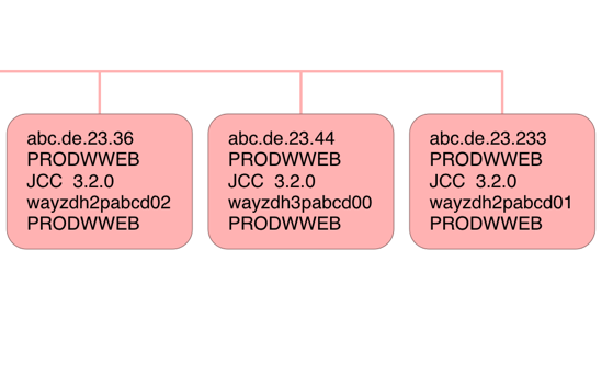
Here are three simple connectors.

The lines in each box are:

• IP Address
• Authid
• Connector type
• Platform
• End User ID

By “simple” I mean that the connection is direct – not via a gateway.

I haven't shown the Netid but for Distributed connectors it is an encoding of the Client Workstation IP Address. While all bar the first character is a hex digit the first is an encoding to make sure the first digit isn't numeric. So “G” means 0, “H” means 1 and so on.

The reason I haven't shown the Netid is that when you decode it this way it's identical to the IP Address – so there is no gateway.

The three connectors (machines) shown have non-contiguous IP addresses so I show them separately.⁵

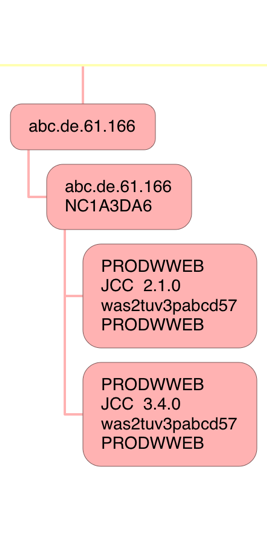
In the above case the JCC level is 3.2.0 but in this data I sometimes see the same machine with two levels:

In this case I show both levels – as separate nodes. Mea culpa: You can see in this case consolidation hasn't been as complete as I'd like, again there being no gateway.

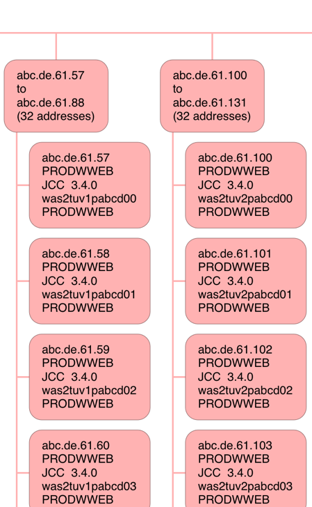
The consolidation of contiguous IP addresses is especially helpful in cases like the following:

I've cut this off after a few addresses – to save you excessive scrolling. But you can see two blocks of 32 contiguous IP addresses, with a fairly obvious naming convention for the JCC Platform ID. I would surmise these are Websphere Application Server machines front-ending the “tuv”⁶ DB2 application.

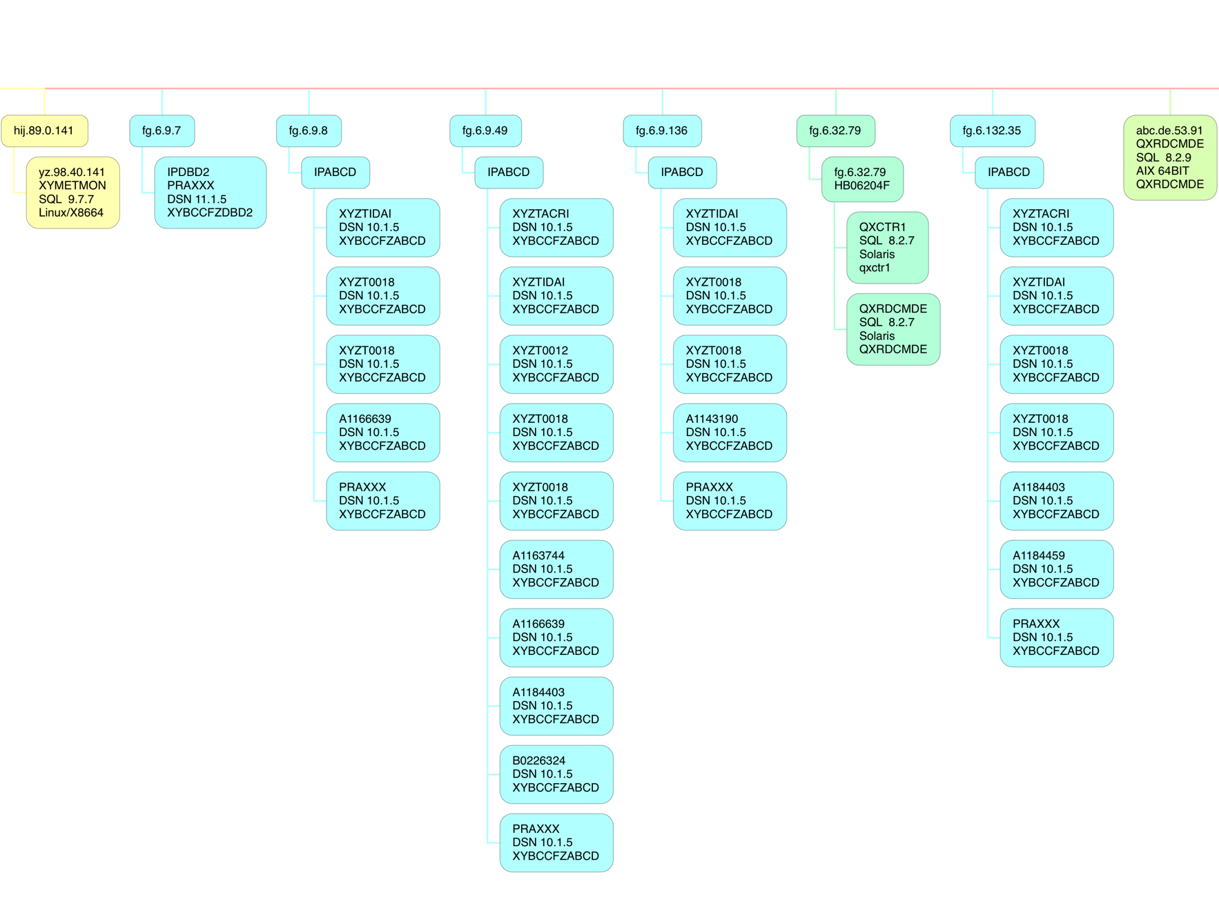
Finally a rather busy one (and you'll want to view this fragment in a new tab):

Here there are several different software platforms:

• 64-Bit Linux on Intel
• DB2 on z/OS
• 64-Bit AIX
• Solaris

And within the DB2 on z/OS category notice “10.1.5” and “11.1.5”. This customer was in transition from DB2 Version 10 to Version 11. Also I recognise 4 client DB2 subsystems at 10.1 – which are the 4 that are in a DB2 Data Sharing group talking DDF to this subsystem (and its Data Sharing Group partners). I bet if I asked the customer those IP addresses would be utterly familiar.

Note also the Netid commonality – “IPABCD” – which I will probably see as a common feature, when I get more experience.

How I Made the Diagram

The process for creating the diagram is two-step:

1. Crunching the data into a Comma-Separated Value (CSV) file.
2. Importing this CSV file into the diagramming application I'm using.

I'll share a few of the specifics with you. If you want to do this you'll need to follow much the same path.

Crunching The Data

Crunching the data, in my case, consists of two batch job steps:

1. A DFSORT step that summarises the 101 records, boiling down to unique names, and preserves the fields needed for diagramming.⁷
2. A REXX EXEC that takes this summarised flat file and generates the CSV file.

I may have mentioned this before but I once wrote a REXX exec to convert this CSV file into Freemind format. I've yet to throw this CSV through the exec but it will be something to try soon.

Producing The Diagram

The process for producing the diagram consists of importing the CSV file into a Mac OS app – iThoughtsX – and a small amount of cosmetic tidying up.

The snippets you see above were actually produced by the counterpart iOS app on my iPad Pro – iThoughts.

Conclusion

While fine tuning the diagram was fiddly creating at least a basic version was very easy.

As always, as I gain more experience with this I'll evolve the diagramming. One obvious thing to do is to highlight the “high volume” or “high CPU” connectors; As I have the data in my flat file it'd be simple to colour code the “hotter” connectors.

One of the nice things to note is a modern tool such as iThoughts allows some quite neat navigation and pattern seeking. For example, I can – in both the Mac OS and iOS versions – use filtering. If I were to type in “mobi” – which appears in the unanonymised version of this diagram – a bunch of nodes will show up and the rest will be grey. This example has obvious application.

For me at least the sorts of insights I can draw into a customer's DDF estate are really nice.

The other nice thing about iThoughts is it has some Presenter capabilities for a mind map such as these; I actually haven't played with that much but I think that could prove really handy.

Perhaps this dinosaur is evolving wings. 🙂

(Originally posted 2017-02-17.)

It's been a long time since I…

… recorded a podcast episode.

But Marna and I have had lots of commitments since we last did. But we're back, and intend to stay that way. Indeed we have bits of Episode 10 “in the can”.

And such a lot has happened in the meantime.

Note: This is actually our tenth episode, though you might count Episode 0 as a pilot and Episode 10 as the real 10th episode. Frankly I don't, as I think Episode 0 is entirely valid. We were certainly learning our craft. What is nice is that people don't seem to have given up on us after that one. 🙂

So, to Episode 9:

In a “packed show” :-), we had all the usual ingredients:

• We had follow up on Continuous Delivery.
• Marna interviewed John Eells on new initiatives in software installation.
• We talked about enhancements to my Parallel Sysplex Performance Topics presentation. (The show notes contain a link to the presentation on SlideShare.)
• Marna indulged me in talking about Voice-Operated Digital Assistants. I've gone “all in” on these.
• She also had a couple of nice requirements.

So I hope you enjoy the show; We had fun making it!

Below are the show notes.

The series is here.

Episode 9 is here.

Episode 9 “Back In Black” Show Notes

Here are the show notes for Episode 9 “Back in Black”. The show is called “Back in Black” because:

• We've been away for a long time, traveling for Martin and on vacation for Marna.

• A vague reference to a BBC tv show about British fantasy author, Terry Pratchett

We are very happy to be resuming our episodes, and the next isn't far behind this one!

Continuous Delivery Follow-up Announcements

• January 10, 2017 IBM CICS Transaction Server for z/OS, V5.3 is further enhanced with the continuous delivery model and the IBM CICS Transaction Server for z/OS, V5.4 open beta offering is updated

• January 19, 2017 IBM Customer Insight for Banking V2.0, IBM Client Insight for Wealth Management V2.0, and IBM Incentive Compensation Management V10.0 follow the IBM Continuous Delivery Lifecycle Policy.

Where we've been

Martin has been all over since our last podcast! Whittlebury UK (with Marna), Amsterdam, Johannesburg, Toronto, Chicago, and the IBM Silicon Valley Lab.

Marna has been to the IBM Technical University in Austin, TX.

Mainframe

Our “Mainframe” topic was an interview with John Eells, z/OS System Test and lead on the Software Installation Strategy.

This topic is very important for z/OS system programmers to understand. IBM and ISVs have been working on a common install method, that handles both SMP/E and non-SMP/E. This would go beyond laying down code, and would eventually hook seamlessly into doing configuration tasks (via z/OSMF Workflow). It would even be able to package software, if you wanted to, and all delivered within the base z/OS operating system.

The common install method would be provided through z/OSMF's Software Management plug-in, so make sure you are setting up and becoming familiar with z/OSMF now.

John and Marna also talked about some of the wishlist items we'd like to see in this solution.

Performance

Our “Performance” topic was about some about additions and changes to Martin's Parallel Sysplex Performance presentation that he's been presenting over the years. Somehow this presentation never seems to get any shorter.

This presentation has several sections: Structure-Level CPU, Matching CF and PR/SM views of CPU, Structure Duplexing, XCF traffic, CF link information, and CF Thin Interrupts.

The new parts and changes he has made in this presentation are:

• Asynchronous Duplexing for lock structures. You can also find a good Mainframe Insights article about this by David Surman here.

• XCF traffic and Data Sharing Group topology

and

• CF Thin Interrupts and CPU.

The updates have been presented in both Munich (at the System z Technical University) and at GSE Annual Conference. Slides are found on SlideShare's Parallel Sysplex Performance Topics from Munich 2016.

Topics

Ahoy! In our “Topics” section we discuss voice-activated assistants that have been hitting the market for a while now.

Martin has a good amount of experience in Siri from Apple and Alexa (Amazon) Echo and Dot. A third one is Google Home.

Martin talks about the various pros and cons on each. Considerations for using these include: inadvertent waking, integration with household devices (such as Philips Hue lights and Wemo switches), extendable capabilities (for Alexa they're called “Skills”) that you can create yourself, what tasks you want it to do, future growth (where competition will help), and country availability.

Customer Requirements

Marna talked about two customer requirements that caught her eye:

• 100505 on developerWorks RFE: Specify DSN HLQ for Healthchecker Debugging

• 100362 on developerWorks RFE:z/OSMF create your own category on left bar

Where We'll Be

Marna will be at SHARE in San Jose, California March 6 through March 10, 2017.

On The Blog

Martin has published three blog posts recently:

• Lost For Words With DDF

• The Suite Spot

• SMT – Some Actual Graphs

Marna has written one: Trying out the new z/OSMF Workflow Editor

Contacting Us

You can reach Marna on Twitter as mwalle and by email.

You can reach Martin on Twitter as martinpacker and by email.

Or you can leave a comment below.

(Originally posted 2017-02-12.)

I'm lost for words with DDF, I really am.

“What's up with him?” my one reader asks. 🙂

So let me explain…

I debuted a presentation last year called “More Fun With DDF”. But I've made progress since then.

So what do I add to the front of this title? “Still”? “Yet”? “Even”?

I don't even think there's a hierarchy to these so it's a one shot deal tacking one of these on the front for 2017. “Even More Fun With DDF” is my favourite of these.

Caveat author! 🙂

So let's get to the meat of it: Something you might actually want to know…

DB2 Calling DB2

So I've been involved in a couple of situations where one DB2 on z/OS calls another, using DDF, recently.

• I'll call the one that does the calling the Client DB2.
• I'll call the one that is called the Server DB2.

The Client DB2 might call the Server DB2 on behalf of anything – such as CICS transactions, Batch Jobs, or even its own DDF clients¹.

For the rest of this post refer to this diagram, summarising key aspects of the SMF 101 (DB2 Accounting Trace) records.

Detecting Client And Server DB2 Subsystems

So how do we detect Client and Server situations?

Firstly the presence of a QLAC section in a SMF 101 (DB2 Accounting Trace) record tells you the 101 represents something participating in DDF – whichever role the DB2 is playing.

Secondly field QLACSQLS tells you this unit of work sent SQL requests somewhere – so it's acting as a Client. Similarly field QLACSQLR tells you it received SQL statements – so its acting as a Server.²

Matching DDF 101 Records

So, if I know that one DB2 is calling another I want SMF 101 (DB2 Accounting Trace) records from both DB2 subsystems. That should help me understand the conversation more fully. I will call these the Client 101 and Server 101 records, respectively.

But how do you match them up?

It turns out that timestamps are useless for this. But Logical Unit Of Work IDs are ideal – well the first 22 bytes of the 24. This is fields QWHSNID, QWHSLUNM, and QWHSLUUV concatenated.

Match these up and you're in business.³

Doing The Matching

I have code that reformats DDF 101s into records with important fields in fixed positions. With this code:

1. I reformat the Client 101s with important information, including the match fields, into fixed positions, with DFSORT COPY.
2. I reformat the Server 101s with important information, including the match fields, into the same fixed positions, with DFSORT COPY.
3. I use DFSORT JOINKEYS to join the two records together, extracting relevant fields from both the Server record and its matching Client record.

Actually I separate Batch, also CICS, also Other DDF joined records into their own data sets. For Batch “blow by blow” is appropriate; For CICS a statistical approach is better. So I have two CSV files, ripe for importing into a spreadsheet, for each of these.

Timings

Timings (and perhaps names) are the payoff for matching up these records.

The first thing to note is that normal (non-DDF) timings apply – in the QWAC and QWAX sections.

That's almost all you need to look at for the Server 101 record. Similarly, for the Client 101 record, the standard time buckets apply.

But there is a field – QWAXOTSE – that documents time waiting for the other DB2.⁴ It works both ways. And when its value is not explained by the 101's time buckets it can indicate communication problems.

Another piece of timing information is the end timestamps – the SMF record cutting time. What I've observed for Batch DDF is that the Server cuts its record a few minutes after the Client. My guess is this is because the Server realises the Client isn't coming back anymore; Some sort of idle timeout. I further suppose the QWACRINV field – the reason for invoking accounting – might provide the explanation But I really need more experience with this. I haven't seen the same effect with CICS DDF transactions, but then the overall numbers are much smaller.

Conclusion

It is perfectly possible to match up Client and Server DDF 101 records; Its value lies in getting a more complete view of such a DB2-to-DB2 conversation, complete with some extra diagnostic capability.

For example, knowing that a Batch DDF step's time is dominated by Synchronous Read I/O Wait in a specific different DB2 subsystem is useful. Or that QWAXOTSE dominates, unaccountably.

So this code is in Production and working fine.

As always, I expect my understanding to grow and the code to get refined. Both things tend to happen with more customer situations and data. You can be sure I'll relate any significant learning points here.

(Originally posted 2017-01-15.)

What is a batch suite?

That might seem like a silly question to ask but it’s inspired by some significant enhancements to our Batch reporting. Dave Betten and I have worked hard on these as time permitted over more than a year.

Traditional Definition Of A Suite

Traditionally, a batch suite is a set of related jobs, usually with some kind of a naming convention that makes them recognisable.

Such a naming convention might be ‘all jobs whose names begin with “XYZ” comprise the XYZ suite’.

Now, following a naming convention like this doesn’t guarantee relatedness. And not all naming conventions look like this. In fact many don’t.

Our Traditional Suite Reporting

Our motivation for reporting at a suite level is twofold:

• Customers understand suites – because that’s how they designed their batch.
• It’s a mid-way point in the hierarchy – between batch service classes / workloads and individual jobs.

So we use suites as a way of structuring the batch conversation.

We produce suite-level reporting (for the past 25 years) comprising such elements as:

• A summary of the suite
• Which jobs in the suite are released together
• Job statistics
• Step statistics
• Job start delays
• Data sets accessed by the suite
• DB2 access by the suite

This set of reports has evolved somewhat over the years, and I’m skipping a lot of the detail.

What hadn’t changed was how we determined which jobs were in the suite: We were restricted to:

• An explicit list of jobs – cumbersome to compile and manage.
• Jobs with a single specific leading character string – in the spirit of “XYZ” above.

Neither of those is entirely satisfactory – so we got to work.

Enhancements To Our Tooling

• As well as filtering on leading characters of a job name we can also filter on trailing characters (which we call “suffixes”).

Originally we only allowed one suffix. Now we allow multiple. For example “D”, “M”, “W”, “Q”.

• We allow filtering on Service Class and Report Class
• We allow filtering on Elapsed Time and CPU Time

As we’ve done this we’ve slowly re-architected the code and tweaked a few things, too. So, for example, we see all the RACF userids and group names.

How This Refines Our View Of A Suite

I guess we’re getting away from real suites with some of this. And this is a good thing:

• A question we get asked a lot is how to reduce CPU – usually for software billing purposes – and so a pseudo-suite called “Big CPU Burners” is really handy.
• When trying to reduce someone’s batch window a pseudo-suite called “Long Elapsed Time Jobs” helps.
• Knowing which jobs are in e.g. “PRDBATHI” Service Class can be useful.

But we also have much more flexibility in defining real suites:

• We have the extensions to job name filtering I mentioned above.
• Sometimes customers will define a Report Class for a particular application.

So I think we’ve made real progress and it’ll enable us to help customers much better.

But I share all this because it might get you thinking about how to analyse and manage your batch estate better, too. For example, making more use of Report Classes to document suites could be handy. That would require cross-functional cooperation – between the people who create the JCL and the schedule and the WLM Keeper.

But a parting word on the value of real suites:

It’s really handy, when doing deeper analysis, to see a job’s predecessors and successors. So a pseudo-suite of “high I/O jobs”, for example, is unlikely to include many neighbours like that.

(Originally posted 2016-11-13.)

Back in the Summer I talked about z13 Simultaneous Multithreading (SMT) in Born With A Measuring Spoon In Its Mouth. I shared that I was feeling my way forward, and discovering others were doing likewise.

Here we are a few months later and my code has come on in leaps and bounds.¹

So I think it’s worth sharing some design stuff and a little discovery; I’m working on the principle that people have to embrace SMT on their own personal journey. ²

So let me show you a couple of graphs. I’ve obfuscated the system names on the graphs but otherwise they are “live”.

Changeable Things Need Graphing By Time Of Day

That is, of course, stating the obvious. But here is my graph that shows how some key metrics vary by time of day:

So, for example, Maximum Capacity Factor – being estimated from live measurements – varies by time of day and workload mix. Obviously, Capacity Factor – representing current load – also varies.

Notice how Average Thread Density – the average number of active threads when any are active – peaks during the day. This is a java-heavy workload, peaking in its use of zIIP during the day.

I’m not yet certain I’m wringing all of the insight out of the dynamics yet but I think this graph a good first step in that direction; My experience of this sort of thing is this graph will evolve a little – as I gain more experience.

Engine-Level Analysis Is Interesting

I’ve been meaning to create this sort of graph for a long time – and SMT provides the perfect excuse.

The x axis is processor (or thread) sequenced by Core ID.³

You’ll notice the general-purpose (CP) processors come before the zIIPs (IIP).

Generating a readable graph but without too many x axis label suppressions is tough. But note for the zIIPS each core has two CPUs (with SMT–2) whereas the CPs have one.

While – from the previous graph – the picture is dynamic I think there is value in this shift-level graph. Doing a 3-dimensional one wouldn’t be hard but I think it would be hard to consume. (Time would be the third dimension.)

In any case there’s some interesting stuff in this graph:

• The Parked processors (in turquoise) are interesting: No GCPs are permanently parked but several are partially parked. For the zIIPs, however, it’s a different story: 6 permanently are – 3 cores. ⁴

• Certain things come in pairs: LPAR Busy and Core Productivity – as they are at the core level, rather than the thread level.

• That’s not entirely true: GCPs don’t exhibit the “paired” behaviour. But that makes sense: Only a single thread is enabled on a core.

• For GCPs CPU Ids are even numbers; For zIIPs they’re both odd and even. The zIIP values didn’t surprise me. The GCP ones did – and I’ve seen this for two customers’ data sets now.

• Some of the zIIP CPU Ids are up in the x’70’ onwards range. This surprised me and caused me to have to widen the CPU Id field to 5 characters. ⁵

Today a lot of the above looks like tourist information. My golden rule with tourist information is there’s high probability it’ll turn out to be diagnostic rather than just interesting – some day.

Conclusion

So, I’m quite pleased with the way these graphs turned out; They do illustrate some of the SMT behaviours.

Obviously experience will condition how this reporting evolves. Watch this (or some similar) space!

(Originally posted 2016-10-29.)

We wanted to get this episode out much sooner, but things conspired against us somewhat. Not least someone we really wanted to interview – to kick off a whole series of topics – having technical troubles.

So we went a different way from what we intended.

And we also had a few scheduling problems. But we’re here now. I hope it was worth the wait.

And just to repeat one thing: If you come anywhere near use we’re miked up. 🙂 Seriously, we’re conducting impromptu interviews when we’re out and about. Find us or avoid us, to taste. 🙂

Below are the show notes.

The series is here.

Episode 8 is here.

Episode 8 “Queue Me Up” Show Notes

Here are the show notes for Episode 8 “Queue Me Up”. The show is called “Queue Me Up” because:

• Marna talks about moving up to higher z/OS releases…or releases “in the queue”.

• Martin talks about the Coupling Facility list structures…or “queues”.

We had some follow up:

• IBM Doc Buddy – available for iOS and Android.

  The latest iOS level is currently 1.1.1. The latest Android level is currently 1.1.2. Still keep an eye out for updates, as they are coming out periodically and delivering requested functions.

• Continuous Delivery Follow-up

  October 4, 2016: A DB2 12 recent announcement includes their Continuous Delivery message, with new functions via the service stream: IBM DB2 12 for z/OS expands the value offered to your business by IBM’s industry-leading mainframe data server

Mainframe

Our “Mainframe” topic was a discussion on z/OS upgrade timing considerations.

z/OS R13 is now out of service since end of September 2016, five years of regular service support since GA. There are three consecutive releases of coexistence (with releases planned on coming out every two years).

This “discrepancy” between five years of service and and six years (three times two) of coexistence has been quite interesting and deserves some thought. Marna talks about some considerations, and it might be that the “n-2” model should be reconsidered to be a “n-1” model for some customers.

Performance

Our “Performance” topic was an extension of this blog post of Martin’s: Right On Queue.

Martin talks about Coupling Facility list structures, and how they are different from lock and cache structures. He also covers some considerations and causes for how they might get filled up. (Think of the analogy of a pipe getting blocked as one case.)

Sizing is important and he uses SMF 74-4 and RMF Monitor III. A good rule of thumb is that your structure’s maximum size should be in the range of 50% to 100% of the current size. More than double puts you at risk of having a list structure full of control blocks and little data. You also need to monitor how much of the current size is actually in use.

Topics

In our “Topics” section we discussed a travel app called Waze. It’s a crowd-sourcing app you can use to get real-time travel estimates and routes. It also alerts you about such items as accidents, debris, police cars, etc, which other users have reported. This app is particularly useful even if you have to put up with a very small amount of advertising.

Where We’ll Be

Martin is in the *shires (Buckinghamshire, Yorkshire, Wiltshire), as well as a short trip to Amsterdam, during the rest of the year (at the time of going to press). And…also with Marna in:

• Guide SHARE Europe UK, November 1-2, 2016. A roving microphone might appear, so please join the conversation if you wish!

Marna is going to:

• IBM TechU Comes to You in Austin, TX, November 14-16, 2016

On The Blog

As well as Right On Queue, Martin posted to his blog since our last episode:

• Automatic for the Peep-Hole – about experimenting with automation for his Apple watch to dictate and send emails – using both web-based and on-device tools. It was really a test bed for thinking about when on-device automation is best and when web-based automation is better.

• Transaction Counts – about counting transactions with RMF.

Contacting Us

You can reach Marna on Twitter as mwalle and by email.

You can reach Martin on Twitter as martinpacker and by email.

Or you can leave a comment below.

(Originally posted 2016-10-22.)

Seasoned readers will recognise the title of this post as a bad pun, rather than a mis-spelling. [1]

One emergent theme in our code for Parallel Sysplex Performance is treating individual coupling facility structures on their merits. For example, lock structures are different from cache structures.

But there is much commonality in the instrumentation. For example Maximum Size, Size and Minimum Size are common to all.

One type of structure I haven’t paid much detailed attention to is List structures. Two common examples are:

• XCF Signalling Structures [2]
• CICS Shared Temporary Storage queues[3]

But an incident recently led me to think about List Structure behaviour:

Two test systems with CICS regions on were sharing a Temporary Storage Queue List structure. The structure itself is 20MB in size (with a Maximum Size of 98MB)[4]

The structure itself got to full.

If you approach the structure as some form of queue it helps, because it lets you muse in the following ways:

• Maybe the reader stopped reading.
• Maybe the writer suddenly splurge wrote.
• Maybe the writer outpaced the reader for some other reason.

The truth of it does need sorting out. All of these are feasible explanations in a testing scenario but you wouldn’t want to go into production like this.

In a queuing environment you have to think about how big a queue is required.[5]

In general a large queue (buffer) helps with transient variations in writer and reader speed; It doesn’t help much with persistent outpacing.

But what can put a “bung” in the pipe? Or appear to?

• A dead reader can do it – whether (in this case) a CICS region, the DB2 it connects to, the LPAR or the machine. You get the picture, I’m sure: It’s not just the actual reader that matters.
• “Market Open” – where a concerted spike in writes can remain unmatched for a while.

So we need to monitor certain list structures. In SMF 74–4 we have, among other things:

• Maximum number of elements – R744SMAE
• Current number of elements – R744SCUE

Plotting the latter as a % of the former is probably the right thing to do. Obviously an RMF interval of, say, 15 minutes might not catch sudden spikes.

But in the “Market Open” type of scenario it’s worthwhile trying to understand what it does to major queues. And as this post is about list structures those would include XCF signalling structures, CICS Temporary Storage queues and MQ shared message queues.

In the case I mentioned, the structure was resized to 49MB. I didn’t hang around to see what the resolution was, from the CICS point of view.

One final thought: Don’t be tempted to set the Maximum Size of a structure ludicrously big, relative to the Initial Size (or even the expected day-to-day size): I have it on good authority the structure would be full of control blocks, rather than data.

(Originally posted 2016-10-09.)

I have to admit to being a bit of a wannabe when it comes to automation.

Certainly most of my career has been built on using and building tools – and you’d have to pry them out of my luke-warm retired hands. 🙂 But when it comes to automation in my personal life it’s a bit of a different story:

• I haven’t (yet) got into Home Automation. Baby steps still.¹
• I don’t use many automation scripts on computers and iThingies.

Now this might surprise some people. But my modus operandi is much closer to “find a real use case” than you might think; I have to find projects that look like they’re close to a pay-off.

Anyhow, I have had a fair amount of practice trying to put workflows together, generally with decent results. Which leads me to slightly abstract musings on the subject of Automation.

In any case, I hope this post is in some small way an eye opener for you as to what you can do with the hardware and software (literally) to hand.²

Having installed Watch OS 3 on my Apple Watch³ I’ve found much to like; The usability, particularly the speed boost and the new dock, has improved to the point I want to play with it much more.

(I also paid a lot of money for a Task Manager that has a very nice Apple Watch interface – OmniFocus – but that’s another story.)

So I’m happy to input text on the Apple Watch – indeed inspired by Omnifocus⁴ – and there are lots of ways to do that. Given that, I thought a nice experiment would be to craft workflows where I can input text on the watch and have that sent as an email to my work email address.

Experiment: Sending An Email To Work

I tackled the exercise of dictating into the Watch and having it email me two different ways:

• Workflow – running entirely on the iPhone and the Apple Watch.
• DO Button by IFTTT and IFTTT – which mostly uses services on the web, kicked off by the Do Button app on the Watch.

One key difference between these two approaches is that Workflow is entirely device-oriented, whereas IFTTT has a heavy dependence on external services. Of course, both approaches require an external agent to actually send the email.

So let’s examine the two approaches in a little more detail.

With Workflow – Solely On iOS and Watch OS

I can rapidly kick off a workflow from the dock in the Watch. The left side below shows the first screen. You can dictate from there. The result is the screen on the right.

If I tap on “Done” the workflow continues, but there’s a twist:

I deliberately (and gratuitously) inserted a stage that gets the phone’s battery level. Obviously this can’t be run on the watch and, more importantly, can’t be run on the web. It has to be run locally and this is the key point:

Automation on the device can pick up things only the device knows about.

Setting up this workflow was very easy – being entirely on the iPhone. To make it work from the Watch I just had to select that as an option.

I will say the folks that make Workflow are very responsive and are rapidly adding to its capabilities.

You can get workflows others have built from within the app, and browse them on the web.

With IFTTT – External Automation

The IFTTT approach is a bit different. For a start you compose recipes using a Web interface, or use ones already built.

Secondly, the trigger for the recipe is a separate app – Do Button.

Thirdly, the action really takes place on the web.

One consequence of web-orientation is that it is device-neutral with an Android client being available. Or even not using a device at all. A couple of my recipes don’t use a device.

Again the action starts in the dock on the Watch.

The left side below shows the first screen of the recipe. The right side shows the dictation screen.

This time I have no ability to insert the phone’s battery level. But that’s not a real-world requirement for me.

I will say I found the recipe creation process a little more cumbersome, but not really difficult.

Again the developers are adding capabilities all the time.

Conclusion

While there’s quite a lot of automation you can do solely on an iOS device – and Workflow is not (quite) the only game in town – eventually most workflows (automation scripts, if you prefer) will need external services. Sending an email is just one of those cases.

But I would counsel people to do as much automation on the device as possible, for three reasons:

• It’s probably easier to develop with e.g. the Workflow editor.
• Security is probably better.
• Speed will be better.
• You can test – and possibly run in “Production” – even when there is no network connectivity. At least up to a point.

But the “on device” and ’fetching out for external services" approaches are not mutually exclusive. For example Workflow has an IFTTT action – where a named recipe can be invoked. It’s just that making good choices as to how to automate pays dividends. And at any given time each mode – on-device and on-web – will have access to different sources of data and actions.

By the way, the screenshots were taken by:

1) Pressing the digital crown and the side button simultaneously.⁵ This stores the screenshot in the Photos app.

2) Using the LongScreen app to stitch the photos together.

Well, I hope I’ve encouraged some of you to play with some nice toys; Despite what I said at the beginning I have a few choice workflows that ease my life.

And I’ll leave it to you to figure out the title. 🙂 It’s a rather contrived pun.