(Originally posted 2016-10-06.)

I’ve been musing on counting transactions for a customer recently. I’d like to share some of that thinking with you.

This post is about RMF SMF Type 72 data, rather than middleware-specific stuff. That’s because it’s

• Generic – applicable to multiple transaction managers.
• Much lighter weight – so every customer can collect, retain indefinitely, and process it.

I’m sure this customer is far from alone in being interested in where growth came from. Because they are a CICS / DB2 and DDF customer I’ll concentrate on that, particularly CICS.

I’ve actually had no IMS situations recently. Also TSO transaction rates are rarely significant in the customers I see, so I’ll ignore TSO.

Batch is quite significant in this customer, but it requires a completely different treatment. Perhaps I’ll write about it some other time.

When I say “growth” it is of course a combination of two factors:

• Growth in transaction rates.
• Changes in CPU time for each transaction.

DDF

I’m going to discuss DDF transactions only briefly; I’ve talked about them a fair amount, not least in More Fun With DDF.[1]

Perhaps more useful is this presentation of mine[2]

But to recap what many people already know: DDF Transaction rate is recorded at the Service Class Period (also Report Class) level – in SMF 72.

This doesn’t really help you when it comes to CPU per transaction. For that – at the DB2 subsystem level – you get DDF transaction rate and Enclave CPU (plus response time). [3]

CICS

CICS is an interesting case, and one I’ll talk about for the rest of this post.

In what follows I’ll refer to the following example, which incorporates a number of typical elements.

If your CICS work is managed to WLM Region goals you don’t get transaction endings.

If transaction Service Classes are used the transaction rate is recorded. [4]

In the example transactions enter through a TOR and progress thence to an AOR. For most topologies the transaction is counted once in SMF 72 even if the transaction spans multiple regions. With SMF 110 CICS Monitor Trace enabled in both the TOR and the pair of AORs, you would see transactions ending in both places. The 110 view of transaction rate would be twice that of the 72 view.

On the subject of growth, for CICS at least difficult to calculate CPU per transaction

• Transaction service classes not same as region ones
  • CPU recorded in region service classes

Difficult To Relate To Business Transactions

How IT transactions are wired together to form business transactions can be difficult to ascertain. In the example there are two business transactions – one in blue and one in green.

Both pass through some intermediate infrastructure, perhaps a web server. Even how non-z/OS transactions turn into z/OS ones can be difficult to ascertain. In our example:

• Business Transaction 1 (in blue) spawns two CICS transactions – which each pass through the TOR to separate AORs the one DB2.
• Business Transaction 2 (in green) spawns a single CICS transaction – which passes through the same middleware components. Possibly it uses the same transaction IDs as Business Transaction 1.

It’s worth keeping an eye on how Applications folks wire together transactions as they can be subject to change; While CPU per CICS transaction might not change the number of them that form a business transaction might.

The trend is towards more complex business transactions – which could mean a heady mix of more CICS transactions and heavier ones.

Difficult To Calculate CPU Per Transaction

As I alluded to when discussing DDF, the CPU per CICS transaction can’t be gained from SMF 72 as the region Service Classes have the CPU and the transaction Service Classes the transaction rate.

If, however, you had a transaction Report Class that corresponded to the region Report Class you would be able to use the data from the two to perform the calculation – CPU from the region Report Class and transaction count from the transaction Report Class.

But what do I mean by this?

If the transactions for a region in a specific Report Class had one of a set of Report Classes that were specific to that Report Class the correspondence could be made.

So, for instance, all the regions for the ATM application have Report Class RRCICATM. The second “R” refers to “Region” and “ATM” refers to the fact this is for the ATM application.

All the transactions that run in these regions have Report Classes like RTCICAT1, RTCICAT2, etc.. When these transactions run in different regions[5] their Report Classes have to be different. Here the first “T” says “this is a transaction Report Class”. “AT1”, “AT2” etc are for the ATM application.

Personally, I think this might be a little fiddly to achieve. But I offer it as a suggestion.

Time To Rework CICS Report Classes?

There are lots of reasons for examining your WLM policy periodically. What I’ve discussed in this post is just another reason to.

Some specific things I’d suggest in this area, for Report Classes, are:

• Make good use of report classes for transactions.

  For example, breaking out Mobile.

• Ensure report class transaction rates add up to the corresponding service class’s transaction rate.

  Unless you’re using Report Classes to aggregate Service Classes they should provide a useful breakdown of the Service Class transaction rate.

• Consider the technique I outlined to relate transactions to regions.

A couple of notes on implementation:

• It’s safe to introduce changes to the Report Class setup one step at a time; There is no impact on performance.
• If you’re tracking through time (and you should) changes to the Report Class (and Service Class, for that matter) setup are likely to introduce problems when comparing “before” to “after”. [6]

In general, though, I would be trying to calculate transaction rates and CPU per transaction on a daily basis, as well as over the longer term.

“Daily” might surprise you but with SMF 72 it’s lightweight and it just might catch an application change that either introduces more IT transactions or makes them heavier.

(Originally posted 2016-09-10.)

Getting back “in the studio” was really nice. And we never had any doubt we’d keep recording – so the title is very tongue in cheek.

Below are the show notes.

The series is here.

Episode 7 is here.

Episode 7 “We Were On A Break” Show Notes

Here are the show notes for Episode 7 “We Were On a Break”. The show is called “We Were On a Break” because:

• It’s been a very long time since we last recorded an episode. You should read nothing into other than our schedules and, in particular, Martin’s long holiday put paid to recording for a while.

  But now we’re back…

We had one piece of follow up:

• IBM Doc Buddy – available for iOS and Android.

  This app has been enhanced with new components (aka libraries) and has received some fixes that users have found. There’s a very reponsive team working on this tool! This app is now better than the old LookAt tool, since reason codes can be searched.

Mainframe

Our “Mainframe” topic was a discussion on Continuous Delivery.

Marna talked about four important references to understand what the z/OS platform is doing for Continuous Delivery. (IBM is embracing Agile development for many new functions, and will be providing those functions to customers in a Continuous Delivery method.)

• March 18, 2016 Redpaper on the z/OS base operating system’s usage of Continuous Delivery: IBM z/OS Continuous Delivery

• May 24, 2016 General IBM announcement on what an IBM product might do for Continuous Delivery: IBM Software Support Lifecycle Policy is enhanced with a continuous delivery support model for eligible, on-premise IBM software products

• April 19, 2016 IBM MQ for z/OS announcement for usage of Continuous Delivery: IBM MQ for z/OS, V9.0 delivers new, more flexible delivery and support options, standards-based messaging support for additional environments, and improved management and administration capabilities. Note “… From this version of IBM MQ onwards, IBM offers a new delivery and support model that separates out the delivery of defect fixes from the delivery of any new function. …”

• July 12, 2016 IBM CICS Transaction Server announcement for some functions using Continous Delivery: IBM CICS Transaction Server for z/OS, V5.3 is enhanced with continuous delivery and the IBM CICS Transaction Server for z/OS, V5.4 open beta offering is introduced . Note “….delivered using the standard CICS service channel..”

Takeaway: some products will be putting their new functions in the service stream, while others might be putting them in releases. Read announcements carefully to see which of your products is following which model.

Performance

Our “Performance” topic was an extension of this blog post of Martin’s: Why Do We Keep Building Bigger Machines?

We acknowledge this is quite a high level treatment but it’s a question that we’re sure has been in the back of lots of minds. We’ve ideas to take some of the subtopics and make them topics in their own right.

Topics

In our “Topics” section we discussed what we (especially Martin) are using for creating presentations these days.

Products Martin mentioned were:

• PDF Pen
• Pixelmator
• Autodesk Graphic
• Powerpoint
• Dropbox
• Box

These are all available in some form or other for both Mac OS and iOS. And, of course, other tools are available.

Where We’ll Be

Martin is going nowhere fast. 🙂 Seriously, his travel plans are relatively local for the next few weeks.

Marna is going to:

• Edge in Las Vegas, Nevada, September 19–22, 2016

• IBM TechU Comes to You in Johannesburg, South Africa, October 4–6, 2016

Interesting Customer Requirements

Here’s two customer requirements we’ve taken notice of. Of course, IBM may or may not decide to do them, but they might be interesting if you’d like to vote on them.

• “zFS Definitions of Greater Than 4 GB Not Being SMS-Managed Should be Available Under IDCAMS”, ID 92523

• “Let IBM Knowledge Center search within a manual and simplify the use”, ID 93288 .

Request for Enhancements (RFEs) can be found here. Most z/OS items are under Brand “Servers and Systems Software”, and Product “z/OS”. Hint: use “I want to specify the brand, product family, and product” when searching.

On The Blog

As well as Why Do We Keep Building Bigger Machines?, Martin posted to his blog since our last episode:

• A Record Of Sorts – about using DFSORT SMF 16 with SMF=FULL creatively to track record counts across job steps.

• Fearful Symmetry – about why things are out of balance.

• Correlation Not Corroboration – about DB2 SMF 101 Accounting Trace Not Accounted For Time.

Contacting Us

You can reach Marna on Twitter as mwalle and by email.

You can reach Martin on Twitter as martinpacker and by email.

Or you can leave a comment below.

(Originally posted 2016-09-03.)

I know of no customer who uses the full capacity of a zEC12, let alone a z13? ¹ So why do we make them bigger each time?

I should state this post is not in support of any product announcement; It’s just scratching an itch of mine.

I think it’s an interesting topic; I hope you agree.

What Is Bigger?

While this post isn’t exhaustive I think the main aspects are:

• Processor Capacity
• Memory
• I/O Capability
• Number Of LPARs

While I’ll touch on these, as examples, I won’t talk much about engine speed; That’d be a whole other post – if I were to write about it.

Where Are Most Customers?

This is just from my personal customer set, but most of my customers are in the range of 10 – 20 purchased processors per machine. Quite a few have sub-capacity processors.

Generally they have two or three drawers (on z13) or a similar number of books (z196 and zEC12). And most of my customers’ machines are either zEC12 or z13, with a few z196 footprints remaining.

Memory-wise, I’m seeing sub-terabyte to several-terabyte configurations, depending mainly on generations.

Customers I work with tend to have two or more machines.

Typically, customers have more than 10 LPARs on a footprint.

I don’t think any of the above is giving away any secrets. And not all customers are like this.

So Why Build Bigger Machines?

There are a number of reasons, which benefit a wide range of customers. Here are some that come to mind.

Scalability

To meaningfully achieve 141 processors (or 10TB of memory) on a single footprint requires good scalability.

I remember, just after the dawn of multiprocessor mainframes, how awful the multiprocessor ratios were. To achieve even modest levels of multiprocessing a lot had to change. And indeed it has, both in software and hardware.

To be able to scale to 141 processors successfully means good multiprocessor ratios are essential. For your 15-way to be feasible, scalability has to be good across the board, all the way up to 141.

The analogy of “the Moon Shot led to non-stick frying pans” is perhaps inappropriate, but the idea that engineering needed for top end machines yields results for smaller machines is sound.

Running Everything On One Surviving Footprint

Bad stuff happens thankfully rarely to mainframe footprints, but when it does customers need to run their high-importance workloads somewhere.

One of the scenarios wise customers plan for is running (the bulk of) two machines’ worth of work on one. Under those circumstances a normally, for example, 20-way might need to become a 35-way. And be effective at it.

So your operating range might need, in an emergency, to be much higher up the scale.

But it’s not just the “machine gone” scenario that has to be catered for. Indeed a subset of the drawers ² in a machine might need to be taken out of service. Then you’d still want to run on the surviving drawers. So, a more powerful physical machine is a good thing, under those circumstances. ³

Unexpected Demand

While the economics of unexpected demand might not be nice, the inability to support a sudden massive increase in workload is even worse.

Most customers I know could grow their workload several times over and still be contained within the same number of footprints.

The trick is to avoid derailment factors. Perhaps “wargaming” massive growth scenarios should be seen in the same light as Disaster Recovery tests.

Two examples:

• The use of the various capacity-on-demand capabilities.
• Middleware scalability e.g. CICS QR TCB.

LPAR Limits

I know customers for whom the (pre-z13) limit of 60 LPARs on a footprint was a real limitation. These are mostly outsourcers.

Several use zVM but it would be nice not to have to ⁴.

I would say a prerequisite to raising the limit to 85 (on z13) was raising the limit on the number of configurable processors way past that. In the distant past I was involved in a Critsit with very large numbers of z/OS images on a footprint.

LPAR design is, of course, critical in this. And Hiperdispatch helps.

Memory

Physically installing memory is one thing; Making it perform is quite another.

For example, we’ve several times changed the fundamentals of memory management in z/OS over the years. ⁵

But note the continuing evolution of the way middleware uses memory.

Also note the way memory pricing has substantially improved over the years.

Closing Thoughts

Workloads are generally growing quite rapidly, mainly through two factors:

• Increasing business volumes
• More being done with each datdatum

So what might today seem very large might seem much more modest going forward.

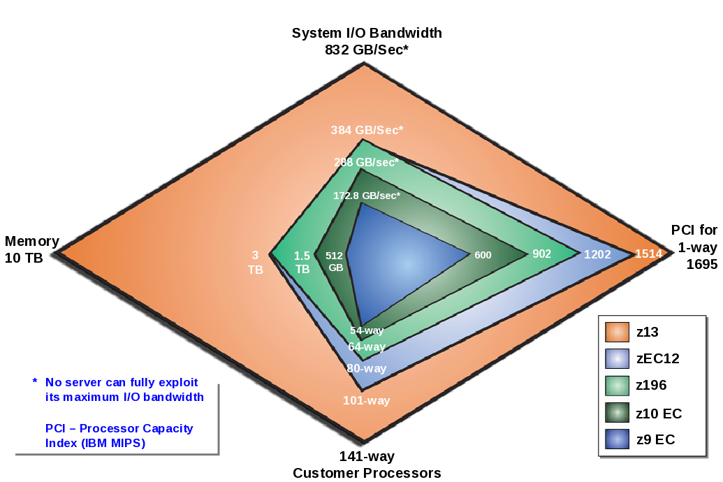
I’ve touched on more than just CPU because configuring systems in a balanced way is important. And you can see we pay attention to that in the following graphic.

This polar chart is for z13 and it shows how over the generations growth has been across all aspects.

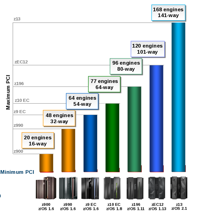
To be specific about CPU, the following chart shows steady growth.

(By the way these two charts were sourced from the most excellent TLLB (Technical Leadership Library).)

We’ve come a long way!

(Originally posted 2016-08-27.)

When looking at a batch job¹ I like to see how the data flows through the various steps.

The first step – some 23 years ago 🙂 – was to look at the Life Of A Data Set (“LOADS” for short).²

With LOADS – for VSAM and non-VSAM data sets – you can see who reads and writes the data set. You can also see the EXCP count. More on that in a bit but suffice it to say EXCP count might be enough to tell you if the data set was written or read in its entirety.

Why Record Counts Matter

Probably just out of curiosity. 🙂

Actually, really not…

I just said I can detect readers and writers and I used the words “in its entirety”. But I think it useful to go deeper. Here are two – off the top of my head – reasons to want record counts:

• Because business volumes can show up in record counts. For example, a transaction file’s record count is the number of transactions in the life of this version of the data set.

• Because it might explain some other count. More on this one in a minute.

Estimating Record Counts

I just used the word “estimating”. Under some circumstances we can do better than estimating, as we’ll see.

One of the reports our “Job Dossier” code produces is called “Job Data Set”. Basically a list of steps and the data sets each step accesses.³

For data sets accessed by QSAM we can estimate the number of records in the data set by examining the LRECL, the Block size and the EXCP count. But there are lots of problems with this:

• This is only going to work for Fixed-Blocked (FB) data sets.
• Compression complicates things. We need to fix our code to handle this – though today we print the compression ratio.
• The assumption is the processing is sequentially start-to-finish.
• You might do a small number of EXCPs not related to actual data transfer.
• It’s likely the step will read or write partially-filled blocks.

Still, where applicable it’s a good start.

But we can do better:

DFSORT’s SMF 16 tells you the overall counts of input records and output records⁴ whether SMF=FULL⁵ or not.

So in a very simple case – a single sort invocation in a step – we can use these record counts to estimate the number of records in the SORTIN and SORTOUT data sets. And we can find the SORTIN data set represented by an SMF 14 record and the SORTOUT data set by an SMF 15 record.

Record Counts And SQL Statements

Several times in a recent batch study the SMF 101 SQL counts have borne some relation to record counts. Consider the following (very realistic) scenario:

The sort step reads a data set (SORTIN DD) and writes one (SORTOUT DD). The DB2 step reads the same data set and does something with DB2 data based on the records read.

For example, in one job step the Singleton Select count matches the input record count.

So we can glean that the selects are record-driven – just with SMF.

By the way, we match SMF 101 records with SMF 30–4 Step End records by Timestamp comparison and Correlation ID matching, which I describe in gory detail in Finding The DB2 Accounting Trace Records For an IMS Batch Job Step. Ignore the “IMS” bit if you like; The preamble is the more general bit.

What My Code Does Today

So, the essential thing is that DFSORT keeps good account of the records written – overall. For output data sets it keeps good counts at the individual data set level (with SMF=FULL).

We map all this, of course.

My first toe in the water is very limited:

For the “single sort in a step with one input data set and one output data set” case I use the SMF 16 record counts as the data set sizes. These overwrite any EXCP / block size / LRECL estimate for FB data sets – as it’s more accurate.

The really nice thing is it gives me an accurate estimate for VB data sets, which I didn’t have before.

Possible Extensions

A number of quite feasible extensions are:

• I could keep the output data set’s record count once I’ve got it and use it in downstream steps. If it gets rewritten then the previous estimate could be invalidated, so that’s safe.
• It would be tricky but I could propagate backwards the input data set’s record count to previous steps that read or wrote the data set.
• I could use the OUTFIL and Output File sections in the SMF 16 record (as we query them) to handle the “multiple output data set” case.
• With multiple input data sets I could pro-rate the input record count across them using the Access Method calls count in SMF 16 Input FIle sections of the SMF 16 record. (This one is dodgy but better than “I’ve no idea”.)
• I said “single sort in a step” but there is enough timestamp instrumentation to do better than that. But where do multiple sorts in a step come from? Here are some examples:
  • DB2 Utilities – where record counts would be especially useful
  • ICETOOL
  • DFSORT JOINKEYS
  • Programs that happen to invoke DFSORT multiple times
• I don’t flag whether a record count is exact – from DFSORT – or estimated. The latter could be printed in italics.

This is quite a long list of potential extensions – but each one is fiddle. Some will get done; Some possibly won’t.

All I know is our code’s ability to estimate record counts took a leap forward, and that is proving useful straightaway. And writing this has helped me sort my thoughts out, as has explaining it to a couple of friends (with a stake in this). And I haven’t even begun to talk about VSAM yet… 🙂

(Originally posted 2016-08-21.)

The title of this post is a Physics reference but this is not about Physics.¹

A customer asked me the question “why am I not getting balanced CPU Utilisation between the various machines”? I’m responding without data at this stage so I’m going to be even more “hand wavy” than usual – both in the long call I had with them and this post.

So, let’s take it in stages…

Why Would You Want Balance?

I think it’s important to put this in context: You’re probably never going to achieve perfect balance, so the real world can’t be an automatic fail.

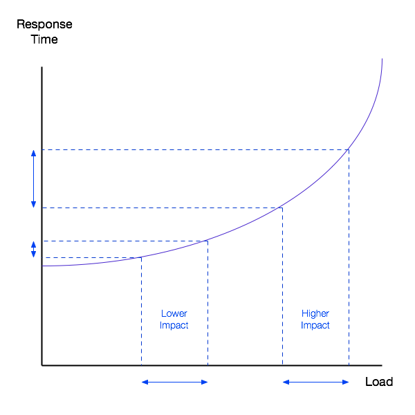
However, there are real world outcomes from imbalance. In the following diagram the impact – however you measure it – is much greater at higher load.

And you might measure it in terms of things like:

• CPU per transaction
• Transaction response time – the example given in the graph
• Batch runtime
• Virtual Storage occupancy

So there can be an impact and that should help you judge what is trivial imbalance and what is substantial.

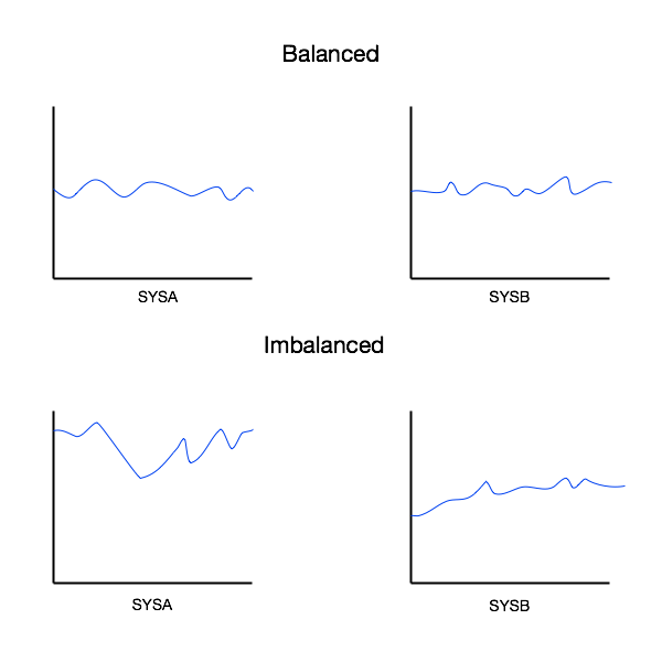
Consider the following two cases:

Obviously in the former case the imbalance – taken as a whole – is not as severe as in the latter case. Momentarily, however, it could be significant ².

There are other considerations:

For example, suppose you have a System Design Point of say 90%. That’s where no system should exceed that level of utilisation. Then significant imbalance (or skew) would cause other systems to have to have a lower maximum utilisation. So upgrades might have to happen sooner.

Where Does Imbalance Come From?

I would divide the causes into two:

• Long-term structural asymmetry
• Short-term routing decisions

Structural Asymmetry

When I look at customers’ mainframe estates I often see symmetric (at a high level) configurations. For example, the “twin machine” architectural pattern is commonplace.

If I dig a little deeper I might see sysplexes spread across these two machines, but additional LPARs on either side that break symmetry.

I might also see the two machines aren’t identical, hardware-wise. For example, one might be a z13 and the other still a zEC12.

Even if the machines are similar enough, their connectivity might not be. For example:

• The primary disk controller might be in the same machine room as one machine, but distant from the other (because the latter is in a different machine room).
• Connectivity to an external coupling facility might be asymmetrical.

Take the case where a sysplex comprise four³ members, two to a machine. I’ve seen cases where these four members aren’t running quite the same workload, in architectural terms. Two examples I’ve seen:

• CICS regions might appear on two members with no analogues on the other two
• Distributed (DDF) DB2 work comes into 2 members of the sysplex but not the other two.
• Likewise asymmetric MQ connections.

Routing Decisions

Work gets routed on a continual basis. I think we can divide this neatly into two:

• Big globs such as Batch
• Smaller pieces of work, such as CICS, IMS and DDF transactions

In principle, big globs ought to be harder to balance than transactions, as should work with affinities. In practice I’ve found this to indeed be so as I’ve had quite a few questions about Batch imbalance.

There are two primary workload distribution systems:

• Round robin, like a card dealer
• Goal oriented, where quality of service influences placement

The former tends to even out the transaction rate, whether work is routed to the optimal place or is indeed CPU-wise balanced. But, statistically speaking, the chances of CPU balance are pretty reasonable.

The latter also has the potential for imbalance, because a better-performing server could well receive the bulk of the work. This imbalance could very well be OK as the aim is to run work well.

Imbalance in the “goal-oriented routing” case is especially a concern with a mixture of faster and slower systems, but this is really a case of Structural Asymmetry, as previously discussed.

How Can I Look At The Data?

The standard “problem-decomposition” approach applies but it’s worth rehearsing it:

• Machine- and LPAR-level configuration and CPU Utilisation from RMF SMF 70
• I/O Subsystem and Sysplex with various subtypes of SMF 74
• Workload-level with RMF SMF 72
• Address Space-level with SMF 30 Interval records
• Transaction level with SMF 101 (DB2), 110 (CICS), MQ (116), 120 (WAS)

All the above is pretty standard and I hope you can see how each of these sets of instrumentation can detect imbalance – whether transient or structural.

Conclusion

So all the above was “talking cure” thinking it through; I suspect actually seeing data would add a whole extra layer of insight and experience.

(Originally posted 2016-08-14.)

This is a post where I have, yet again, to be careful to obfuscate the customer’s situation; I’ve no wish to embarrass them. So you’ll forgive me if there are no numbers. But there is a lesson worth sharing here. So I’m going for it…

It’s about DB2 and Workload Manager.¹

I was recently asked to explain why an application’s DB2 Accounting Trace was showing so much Not Accounted For Time² (NAT). Willie Favero discussed this here, essentially pointing to this IBM Technote.

There are a few things I’d pull out from this document:

1. It’s part of DB2 Class 2 time – so when DB2 is supposed to be in control.

2. The main causes are CPU Queuing and Paging. But there are a lot of others.

3. It talks about NAT usually being small but I’d have an open mind about that. My experience is it is often quite large.

Point 2 is worth exploring in this case:

The umpteen others are generally not the cause of NAT, so I tend to advise customers to concentrate on CPU Queuing and Paging as potential causes.

So, while discussing this with the customer, the following occurred to me:

Let’s look at this from a WLM point of view

Before we go too far with this, it’s important to understand where DB2 work gets classified in WLM terms.

While there is some work that gets classified as DB2 – the subsystem address spaces in their Service Classes – the vast majority of DB2 work runs with the Service Class (and Dispatching Priority) the original work was classified with. For example:

• CICS transactions with the CICS goal for their region (or one derived from the Transaction ).
• DDF work classified via its own rules – into Enclaves in the DB2 DIST address but still not with DIST’s Service Class / Dispatching Priority.³

So, the point of this post is to make the linkage between WLM Goal Attainment and DB2 NAT.

To keep this simple – and the actual customer case looks like this – let’s assume we’re talking about a CICS application with regions classified with Region goals, going against a DB2 subsystem.

Region goals are Velocity goals, which makes the following make sense…

Suppose the Velocity goal is Importance 2, Velocity 60%.⁴

Given velocity attainment is

you could have quite a lot of Delay For CPU samples and still make the goal. So long as there were no other Delay samples, such as Delay For I/O.

And, you probably guessed this part, this level of Delay For CPU is going to appear as some level of NAT.

Corroboration Not Correlation

At this point I flatter myself to think you’ve been wondering where the title comes from. 🙂

So let’s get to it…

I don’t think you can take the WLM view (from RMF Workload Activity Report / Data) and use the numbers therein to derive Not Accounted Time (NAT). So you won’t get Correlation.

But I think you will get Corroboration: A large amount of WLM Delay For CPU will probably happen at the same time as a large amount of NAT.

And that’s really all that’s needed.

To finish this off, let’s look at some wrinkles:

• There are other Delay sample types, such as Delay For I/O, that aren’t related to NAT. (Paging, however, is related to it.)
• It might be difficult to summarize DB2 Accounting Trace over any given WLM Service Class. Note: Apart from DDF the 101 record doesn’t contain the WLM Service Class.
• Delay For CPU might hit other things, such as non-DB2 CICS transaction processing.
• Likewise the non-DB2 portion of a DB2 / CICS transaction, where it would show up in Class 1 minus Class 2 time.

So, this was an interesting question to be dealing with but it’s not entirely “clean”. The upshot, however, is that if you see lots of Not Accounted For Time in DB2 Accounting Trace it’s worthwhile looking at the WLM (or even System) perspective.

And we’re definitely in the Corroboration not Correlation space, and certainly not Causation.

(Originally posted 2016-08-11.)

(Reposted without change as I accidentally deleted it while getting rid of a SPAM comment.)

Episode 5 had a different feel for me. It was our first “trip report” episode, and it felt much looser for that.

In fact the sound effects between topics could’ve been elided but for now I’m sticking slavishly to the format. It didn’t feel too artificial to me.

I’m conscious that most of my readership and our listenership (and the stats prove you exist, as I said in the show) weren’t in Munich.

I think, though, there are things that non-attendees will find valuable or at least enjoy.

People probably think I like the sound of my own voice; The reality is I’m coming to like it. 🙂 Nobody likes how they sound recorded. But the conventional wisdom – that you get used to it – seems to be true.

Thanks to our friend Margaret Moore Koppes for “playing Paparazzi”. 🙂

And the audio production gimmick is subtle this time. 🙂

Below are the show notes.

The series is here.

Episode 5 is here.

Episode 5 “The Long Road Back From Munich” Show Notes

Here are the show notes for Episode 5 “The Long Road Back From Munich”. Here is the link back to all episodes: Mainframe, Performance, Topics episodes.

The show is called “The Long Road Back From Munich” because we’ve both returned from a successful z Systems conference 2016 IBM z Systems Technical University, 13 – 17 June, Munich, Germany. For one of us the journey was much longer back than for the other one.

Mainframe

Our “Mainframe” topic was Marna’s z/OS observations from the conference:

• *IBM HTTP Server Powered by Apache*: it seemed about 30–40% were impacted by the move from the Domiino to Apache server. More than hoped, but if you work on it while on z/OS R13 or V2.1, you’ll be well-positioned for z/OS V2.2.

• *zEvent sessions*: Martin and Marna both went to Harald Bender’s zEvent session where he discussed using your mobile device (either Apple or Android) to receive timely information about events on your z/OS system. The handouts are here: zEvent and z/OS Console Messages to Your Mobile Device . This app was so easy to download and start using, Martin did just that during Harald’s session!

• *z/OSMF*: Marna was happy with the interest in z/OSMF, and with the z/OSMF V2.2 enhancements rolled back into z/OSMF V2.1 in PTFs from January 2016 PTF UI90034.There is no reason to delay using it. The z/OSMF lab for SDSF, however, had a problem as CEA had gotten its TRUSTED attribute removed somehow before Munich. After it was made TRUSTED (after the conference), everything was fine again. Goes to show how important the security settings are for z/OSMF!

• *z/OS V2.2*: Good interest in the release. Happy to see so many people already running z/OS V2.

• *Secure electronic delivery*: Since regular FTP for electronic delivery was removed on March 22, 2016, only secure delivery is available. No one at the conference said they were impacted, which was nice to see.

Performance

Our “Performance” topic was Martin’s performance observations from the conference:

• *State Of SMT Instrumentation Knowledge*: Simultaneous Multi Threading (SMT) metrics are not well understood at this point. Customer data from turning on SMF (for both zIIP and IFL) is starting to appear on Martin’s desk. The good news is that the pickup on this function is fast.

• *His Presentations*: Martin’s sessions were nicely attended. Martin is continuing with his fun at looking at DDF, and “He Picks on CICS” might have more information to be added in the future.

The presentations can be found on Slideshare:

• He Picks On CICS

• More Fun With DDF

• Parallel Sysplex Performance Topics

• How To Be A Better Performance Specialist

Topics

In our “Topics” section we discussed various other conference observations:

• *Martin presented sessions from his iPad.*: Although a lot of cables had to be carried around, it did work fine. He even used his Apple Pencil to mark on the slides during his presentations. So he might never lug a laptop to a conference again. Famous last words!

• *Conference poster sessions*: What a success! Martin & Marna had a poster about…wait for it…this podcast. Martin was very busy talking to people who were interested in our poster. Marna also had a poster on using MyNotifications for New Function APAR notification: New Function APAR Notifications .

  We tried out a QR code for our podcast, and it worked for most all people.

  Paparazzi were there to take photos of some famous folk that stopped by the poster sessions: .

Where We’ll Be

Martin is taking a well deserved vacation for July, so there’ll be no new podcast episodes in July. But we promise to return early in the Autumn!

Marna is going to SHARE in Atlanta, August 1–5, and IBM Systems Symposium in Sydney Australia (August 16–17).

On The Blog

Martin posted to his blog, since our last episode:

• Born With A Measuring Spoon In Its Mouth
• Engineering

Contacting Us

You can reach Marna on Twitter as mwalle and by email.

You can reach Martin on Twitter as martinpacker and by email.

Or you can leave a comment below.

(Originally posted 2016-07-11.)

Episode 6 was a complete surprise to us!

Marna had thought I was on vacation a week earlier than I was. To be fair, I expected to be with a customer in Australia that week. But then the workshop got pushed back and so this week came free [1]

So we went “why not?” and so this episode was born.

It is of course largely built around this blog post but we had a couple of other things we want to say.

And I wanted Marna’s take on the topic.

Talking of the other topics, it’s occurred to me the QR Code capability in zEvent 3.0.0 could be a thumpingly good way of setting up subsequent devices with the same Connection URL.

And the audio production gimmick is accidental this time. 🙂

Below are the show notes.

The series is here.

Episode 6 is here.

Episode 6 “Expect The Unexpected” Show Notes

Here are the show notes for Episode 6 “Expect The Unexpected”. Here is the link back to all episodes: Mainframe, Performance, Topics episodes.

The show is called “Expect The Unexpected” for two reasons:

• We really didn’t expect to be recording an episode in this timeframe.
• The Performance topic lends itself to such a title.

We had one piece of follow up:

• IBM zEvent has been updated to 3.0.0 (“The Cat”) on both Android and iOS. It has enhancements in lots of areas. The one we both noticed was the ability to show and scan QR codes for connections.

Mainframe

Our “Mainframe” topic was a discussion on IBM Doc Buddy – available for iOS and Android.

It’s a tool for looking up error messages and is now enhanced with z/OS Unix Reason Codes. It enables retrieving z Systems message documentation and provides the allows you to look up message documentation without Internet connections after downloading desired files.

It’s available for z/OS, as well as other products like CICS, and IMS, and for many releases of those products.

Performance

Our “Performance” topic was about what happens when unexpected work appears on your beloved mainframes. A number of themes were discussed, including:

• Not knowing mobile workload was appearing – leading to potential loss of savings on Mobile Workload Pricing.
• When unannounced work arrives, leading to implications for e.g. Security, Performance Management, and Capacity Provisioning.

In reality how you handle this is a governance and culture question, but we want you to think about the problem.

Topics

In our “Topics” section we discussed two items:

• iTunes – where you can now find our podcast here. We hope some of you find this new way to subscribe easier.
• Liberated Syndication (or LibSyn for short). This gives us some interesting statistics about our listenership.

Where We’ll Be

Martin is taking a well deserved vacation for July, so there’ll be no new podcast episodes in July. But we promise to return early in the Autumn!

Marna is going to SHARE in Atlanta, August 1–5, and IBM Systems Symposium in Sydney Australia (August 16–17).

On The Blog

Martin posted to his blog, since our last episode:

• What Do I Know?

Contacting Us

You can reach Marna on Twitter as mwalle and by email.

You can reach Martin on Twitter as martinpacker and by email.

Or you can leave a comment below.

(Originally posted 2016-07-02.)

Or “The Man Who Knew Too Little”?

This post is occasioned by a number of things coming together, the most recent of which is reviewing a very nice upcoming RedPaper.

The gist is this: You’re responsible for managing Performance, Capacity and (to some extent) mainframe costs. But you can’t rely on anybody to tell you anything.

A bit pessimistic, perhaps a little misanthropic. But still something I’m sure a lot of you can relate to.

There are two major exemplars that cause me to write this post:

• Mobile
• Cloud

There, I’ve got two buzzwords into a post. 🙂

But let me take each in turn.

Mobile

My main interest in mobile work is the potential for customers to take advantage of Mobile Workload Pricing (MWP).

Entirely correctly, people are exercised by the need to “Tag and Track”:

• Tag means labelling the work as Mobile, whichever application architecture you choose.
• Track means using the tagging to report the Mobile CPU.

I would add a third (or rather a zeroeth 🙂 ) one: Identification. And herein lies the problem…

Since the announcement of MWP I’ve been taking soundings with customer friends: I’ve asked them “If someone introduced new mobile workload to your systems would they tell you?”

Maybe I’m being humoured but their take has been “not necessarily”. I’m inclined to believe them.

The implication of any non-reporting is clear: Opportunities to exploit MWP might be missed. And one implication of that would be z/OS is unnecessarily less competitive than it might be. I certainly don’t want that.

One thing to note is I don’t think you can assume you’d detect new mobile work, nor to discern its eligibility for MWP in any automated fashion. But I hope you would detect new work showing up.

Cloud

Cloud presents a different problem:

On z/OS the usual approach to cloud deployment is not to create new LPARs; Rather it’s to deploy new subsystem instances, such as MQ queue managers, DB2 subsystems and CICS regions.[1]

With modern tools, such as z/OSMF and UrbanCode Deploy it’s ever easier to create new groups of address spaces – in response to some business application need.

While I’d never advocate making things unnecessarily difficult, making them very easy might have an unintended consequence: Not enough attention to the implications of deployment.

So, for example, the memory footprint of a new DB2 subsystem, another MQ queue manager, and a bunch of CICS regions could be significant. Yes, modern machines tend to have tons[2] of memory but it still needs to be provisioned and managed.

I haven’t done Security for over 25 years but I would suspect there’d be companion concerns there, too.

The good news here, though, is you can detect new containers and their interconnectedness. I’ve written about the SMF 30 Usage Data Section extensively. (If you haven’t picked up on this read this 2012 post of mine.

Mobile and Cloud Have Much In Common

Both these cases are examples where work can show up on your beloved z/OS systems with no warning; You’re expected to handle it optimally.

It’s not often I write about such an “up-market” topic as Governance [3] but I think this is what is called for.

Your processes for onboarding work are what’s important here:

• It needs to be the culture that new work arriving needs some sort of review.
  • For Mobile business application owners need to understand the opportunity for cost savings if they enable you to Identify, Tag and Track work.
  • For cloud it shouldn’t be the case that the ease of deployment leads to unannounced “new arrivals”.
• Detection and tracking – to the extent possible – is key.
• Architecture remains important: A hodge-podge of new applications, without considering architecture, is not what’s really wanted.
• The above sound like “policing”. More positively, Performance Tuning and proper Resource Provisioning can make a big difference to how well the business owners view the successive of the deployment.

I don’t know anymore if my readership is confined to (bemused)[4] Performance People. I would hope it would now include architects. In any case y’all are key to successfully managing cloud and mobile workloads on z/OS.

Game on!

(Originally posted 2016-06-11.)

Pardon the bad pun. Perhaps I should’ve written “Engine-ering” but where exactly do you put the dash?[1]

There were hints on this topic in Born With A Measuring Spoon In Its Mouth but the real motivation came from a z196 customer without Hiperdispatch enabled.

But what on earth am I on about?

OK, here we go:

Generally our[2] code doesn’t report down to the single engine (or processor) level.

• SMF
• Hiperdispatch

Actually the same customer who isn’t using Hiperdispatch is using IRD [3], a predecessor and third case where engine-level reporting could be handy.

Why We Don’t Generally Go Down To Engine Level

We generally stop at pool (or processor type), for example the zIIP pool.

Traditionally there hasn’t been much you can actually affect at the engine level.

So the sorts of questions we ask are:

• How busy is the IFL Pool?
• How much CPU in the GCP Pool is this LPAR using?
• Which application componentry is using the zIIP capacity?
• How busy is a Coupling Facility?

None of these are helped much by going to the level of an individual engine.

Why We Might Be Interested In Engines

LPAR design has always been interesting (and a little tricky).

It’s got worse[4] with the advent of such things as IRD, Hiperdispatch and “high stringency” zIIP users[5].

So, to take one example, Hiperdispatch Parking behaviour is an engine-level phenomenon most customers need to understand and monitor.

Theoretically, if we were interested in certain kinds of contention, seeing a skew in favour of, say, one engine might be interesting.

Where Are We Starting From?

Let me lift the lid on where our code is (just a little):

• In table (record mapping terms) we go down to the engine level for all RMF record types. We roll up from there.
• in reporting we handle IRD and do some Hiperdispatch work. See below.

IRD Reporting

We graph shifting weights within an LPAR Cluster. Our view of what the weights say the number of shared engines for an LPAR should be is dynamic.

We graph the number of online engines for an LPAR. When IRD was in its heyday this could be quite interesting.

Hiperdispatch Reporting

We look at two things:

• Vertical Polarisation
• Parking

A couple of posts of potential interest are:

• A Parked Topic
• IRD And Hiperdispatch – Wrong ’Em Boyo

Engine-Level Data Model

The engine-level data model is pretty extensive. There are two cases to consider:

• Coupling Facility View Of CPU (SMF 74–4)
• General View

Coupling Facility Engines

I already dealt with the CF view in Shared Coupling Facility CPU And DYNDISP. You might not have read it – if you don’t have Shared ICF engines.[6]

In the post I mentioned R744PBSY and R744PWAI – “Busy” and “Wait” times. What I briefly mentioned is that these are recorded at the logical processor level.

My current take is there’s only limited excitement to be had by reporting at the engine level – given L-shaped ICF LPARs are a thing of the past.

So, right now, our log table does indeed have Processor Number (R744PNUM) as a key. Our summary table (the one we actually report from) doesn’t. I don’t intend to change that.

General View

SMF 70–1 gives engine-level information in quite a few areas:

• I previously mentioned Online Time (SMF70ONT) in the context of IRD.
• For Hiperdispatch we have Polarisation flags – For High, Medium and Low engine cases. We also have Parked Time (SMF70PAT) but only for the reporting LPAR’s processors (which I first wrote about in 2008 in System z10 CPU Instrumentation).
• At the LPAR level we have the Logical Processor Data Section
• For SMT we have all I mentioned in Born With A Measuring Spoon In Its Mouth.
• We have CPU busy by engine for the reporting LPAR in the CPU Data Section.

The Shape Of Things To Come?

So what am I thinking of?

Well, the underlying principle is that it’s the non-uniformity between (logical) engines for an LPAR that is interesting.

And maybe – in another dimension – how that non-uniformity varies through time.

So I’ve run a couple of experiments with recent customer data:

• A Non-Hiperdispatch Case.
• A Hiperdispatch Case where the GCP Engine Pool is extremely busy.

I don’t have to hand the case where Hiperdispatch is in play but the GCP Engine Pool is not busy. I have thoughts on what might happen, but this post is already running long.

Non-Hiperdispatch Case

In this case the LPAR is defined with 8 Online GCPs and 10 Online zIIPs -on a z196.

Here work is “smeared” across all the online engines, certainly the GCPs. None is more than half full, and typically they’re about a third full.

This has effects, such as short engine effect. Also the cache effectiveness won’t be wonderful.

Hiperdispatch Busy GCP Pool Case

In this case the LPAR is defined with 10 Online GCPs (6 Vertical High, 2 Vertical Medium (at 65%) and 2 Vertical Low) and 2 Online zIIPs (both Vertical Medium (at 80%)) – on a z13.

Here, the work is “corralled” into just the Vertical Highs and Vertical Mediums, in accordance with the vertical (engine-level) weights. We are approaching full engines – quasi-dedicated to the LPAR – for the VH cases. There is some evidence of parking and unparking of the Vertical Lows.

So What Might I actually Do?

I can certainly generate graphs like the above at will – and I probably will.

I’m more inclined to do it for the system under study than for all LPARs on a machine / in the data for three reasons:

• It’d be an awful lot of graphs for most of my customers. And the value for obscure LPARs wouldn’t be huge.
• If I have SMF 70 cut by an LPAR (really z/OS system) it will also contain Parked Time (SMF70PAT). Relating Parked Time to Engine Busy Time will be interesting.
• Keeping core vs logical processor straight is important, and driving the above graphs down to logical level is useful. It can only really be done for the systems I have data from.

All the above sounds a little undecided to me – and it is. The reason for sharing all this is because I think Engine Level could well prove useful, as well as being interesting. And, not having seen much writing on this, I suspect this is something most Performance and Capacity people won’t’ve thought about.

I for one intend to keep thinking about this and experimenting. Stay tuned. 🙂