(Originally posted 2016-06-05.)

SMT really was born with a measuring spoon in its mouth.[1]

Let me rewind a few years…

So, when SMT (Simultaneous Multithreading) was being designed I was privileged to be on the periphery of discussions about how to instrument SMT. Things like CPU Utilisation get a little wierd in the SMT case, as you can imagine.

Now, I was only on the periphery of the discussions and they carried on without me in the run up to the announcement of z13 in early 2015. But the drift I caught was that the hardware was going to have to help out, essentially being self-metering.

Fast forward to now, just over a year after we first shipped z13. And now I come to warm over our CPU code to account for SMT.

Timely, huh? 🙂

Seriously, from where I sit I have to see real data from real customers before I can do serious development.[2]

Now, in mid–2016, there are lots of z13 customers. So it’s time to act.

Remember that SMT “only” affects zIIPs and IFLs. GCPs and ICF engines are not affected. So everything already works fine for GCPs. But obviously hiding behind the fact it’s only certain types of engines that support SMT is not a good thing to do.

Rewind again, but this time to the Autumn of 2015. I had the privilege of presenting a one day workshop on Performance for the ITSO in Europe.

A smallish section of this was about SMT, and an even smaller portion of it was about the measurements. So what I really wanted to impart with that material was the general sweep of the instrumentation; That some stuff was on a per-core basis and some on a per-logical-processor basis.

Now a core is the thing that can have multiple threads and it’s basically all PR/SM knows about. It’s z/OS that knows about logical processors or threads.

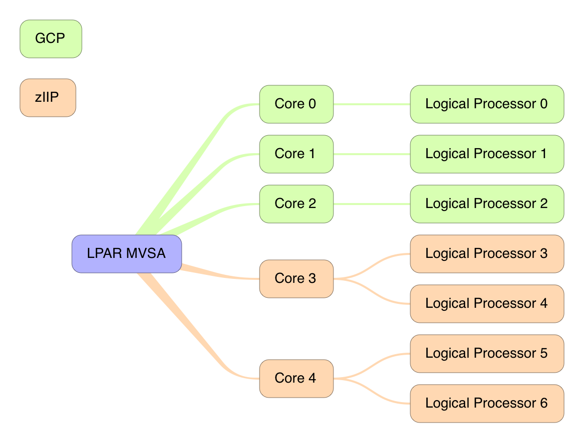
Here’s an example[3] that might explain the relationship between logical processors and logical cores:

In this example MVSA has 5 logical cores.

• Logical cores 0,1, and 2 have a single thread and are GCP cores.
• Logical cores 3 and 4 have two threads and are zIIP cores.

So SMT–2 clearly affects zIIPs and not GCPs, as the diagram shows.

Obviously logical cores get dispatched on physical cores by PR/SM.

In the workshop I showed (briefly) sample RMF reports – for PROCVIEW CPU (non-SMT) and PROCVIEW CORE (SMT 1 and SMT 2). By the way the support in RMF came with OA44101.

Back To The Present

Returning to the present moment I want to replicate that, and then put my own personal twist on it.

(Generally that’s the way to go: Replicate RMF and then progress beyond the product’s reporting.)

So, for most major numbers in an RMF report you have to derive them. The nice surprise with the SMT support is that the numbers are basically there. By “basically” I mean the worst you have to do is divide by 1024.[4]

So, for example the following fields are all there in the SMF 70–1 record (in the sole CPU Control Section).

• Maximum Capacity Factor
• Capacity Factor
• Average Thread Density

You get one each for GCPs, zIIPs and (gasp!) zAAPs.

I mention these by name in the hope the astute reader will recognise them as terms used in most performance materials related to SMT.

But the point is that no fancy derivation is necessary.

What Else Is New And Changed In SMF 70–1 For SMT

First the CPU Data Section (previously one per logical processor) is at the thread level, not the core level. (In fact, thread is synonymous with logical processor.)

So this now needs relating to the core. Here’s where the next change comes in: The new Logical Core Data Section.[5]

This has a number of aspects:

• It allows you to relate the logical processor / thread to the core.
• You get the Core Productivity number.
• You get the Core LPAR Busy time.

A question you’d probably like to be able to answer is “which LPARs on this machine have PROCVIEW CORE in effect?” The answer to this is found in the PR/SM Partition Data Section (one per LPAR): If field SMF70MTID is greater than 0 PROCVIEW CORE is in effect; Otherwise it’s PROCVIEW=CPU.

Finally, in the PR/SM Logical Processor Data Section (one per logical core) SMF70MTIT gives you the “Multithreading Idle Time in microseconds accumulated for all threads of a dispatched core. This field is only valid if SMF70MTID is not zero for this partition.”[6]

A Lot To Chew On

If you’d come to the conclusion there’s a lot to chew on here you’d be right. But at least we’re being spoon-fed.

To continue the malaphor, I’m still digesting this; The definitions are a little hazy in my brain, but at least I have a way of seeing how the data behaves in real customers.

And I have some thoughts on how to diagram things (as the picture above illustrates) and otherwise tell the story. More on this as I implement in my code; For now things are going to have to be hand-drawn.

Happy chomping!

And here’s a nice presentation on SMT to digest: IBM z Systems z13 Simultaneous Multi-Threading (R)Evolution by Daniel Rosa, IBM Poughkeepsie.

(Originally posted 2016-06-04.)

Episode 4 was, of course, our fifth podcast episode. 🙂

I had a lot of fun making the intro – with Audacity. I’m not sure if it’s “lost souls” or “tuning in”. It was meant to be the latter but the former is also good.

Below are the show notes.

The series is here.

Episode 4 is here.

Episode 4 “The Road To Munich” Show Notes

Here are the show notes for Episode 4 “The Road To Munich”. Here is the link back to all episodes: Mainframe, Performance, Topics episodes.

The show is called “The Road To Munich” partly in homage to the Road To… movies and partly because we’re preparing for the 2016 IBM z Systems Technical University, 13 – 17 June, Munich, Germany.

Follow Up

Following up the Episode 3 “Topics” item on iThoughts and Mind Mapping, Martin wrote up how to make a (colour-coded) legend in iThoughts The Legend on his blog.

Mainframe

Our “Mainframe” topic was on a small z/OS V2.1 enhancement that few seem to be using: SMFPRMxx’s AUTHSETSMS. This new option controls whether you want to allow use of the SETSMS command, different from the SET SMS command, without tying it anymore to the specification of PROMPT. Exploiting this function is as easy as adding AUTSETSMS to your SMFPRMxx for the next IPL!

Performance

Our “Performance” item was a discussion on another of Martin’s “2016 Conference Season” presentations: “He Picks On CICS”.

We’ll publish a link to the slides when they hit Slideshare, probably after the 2016 IBM z Systems Technical University, 13 – 17 June, Munich, Germany.

Topics

Under “Topics” we discussed Uncharted 4. The Wikipedia entry is here.

On The Blog

Martin posted to his blog, in addition to the previously-mentioned item:

• Shared Coupling Facility CPU And DYNDISP
• Refactoring ISPF File Tailoring And DFSORT
• More Fun With DDF

Contacting Us

You can reach Marna on Twitter as mwalle and by email.

You can reach Martin on Twitter as martinpacker and by email.

Or you can leave a comment below.

And we hope to have a poster session in Munich. Join us then or come and stop us any time you like that week.

(Originally posted 2016-05-29.)

You probably don’t have the same problem I do, namely not having access to SMF data from all the systems in your mainframe estate.

You’ll recognise that as a provocative statement if ever there was one; For all sorts of reasons not every system’s RMF SMF is collected.

Most notably, test systems often aren’t instrumented.

This post is about Coupling Facility (CF) image CPU. Mostly it’s about CF images on the same footprint as a z/OS system for which you do have data. [1] The discussion is limited to CPU.

So there are two views of Coupling Facility CPU:

• SMF 70 Partition
• SMF 74–4 Coupling Facility

Both of these are available at the partition and engine level, but the latter is less interesting.[2]

Coupling Facility CPU Utilisation Might Not Be What You Expect

So a standard formula for Utilisation % would be, summed over all engines:

From an SMF 70 perspective that’s certainly true, but it’s not how CF CPU Utilisation is calculated. It’s the following formula , summed over all the engines:

Now, the two formulae look similar, and they would be the same if R744PBSY+R744PWAI added up to the interval length. Well, this is true only for dedicated CFs, namely those not sharing engines with other LPARs.

So for dedicated LPARs that’s fine: CF view of busy (74–4 view) is the same as PR/SM view (70–1 view).

What Are R744PBSY and R744PWAI?

R744PBSY is the CPU time (in the CF) processing requests – from all systems.

R744PWAI is the CPU time (in the CF) polling for requests to process.

With DYNDISP=NO R744PBSY+R744PWAI do indeed add up to the interval x the number of engines as the CFCC never stops polling for requests.

With DYNDISP=YES they don’t add up to the interval x the number of engines. This is because the CFCC stops polling for requests, but not immediately.

So the formula for CF utilisation is really about what percentage of the CF CPU cycles is used processing requests.

What Is R744SETM?

I first wrote about this field in 2008 and you might get a snigger at my expense. Readers in 2008 did. 🙂 Here’s the post: Coupling Facility Structure CPU Time – Initial Investigations

It’s the Structure Execution Time, or CPU time in the Coupling Facility for a CF structure. Key points about it are:

• R744SETM is for all systems accessing the structure.
• R744SETM adds up to R744PBSY

Because of the latter its capture ratio is 100%. This has an effect at low traffic rates; There appears to be some CPU utilisation without any requests. But the CPU per request tends to settle down.

As I said in the above-referenced post the CPU per request [3] calculation relies on having data from all systems sharing the structure.

Standard Recommendations Still Apply

It’s still wise not to run coupling facilities above 50% (according to the SMF 74 formula). This is for two primary reasons:

• The CF needs to be as responsive as possible, as it affects Coupled CPU. (This includes link times, of course.)
• You might well need “white space” for recovering structures (or, in the case of User-Managed Duplexing, for the Group Buffer Pools to become primary).

What Of Coupling Facility Thin Interrupts?

So now I’m coming to the point[4].

System zEC12 and CFLEVEL 19 introduced Coupling Facility Thin Interrupts, enabled with DYNDISP=THIN.

Barbara Weiler has a nice paper on this: Coupling Thin Interrupts and Coupling Facility Performance in Shared Processor Environments, so this post is covering only a small (but relevant) portion of what she covers.

In essence Thin Interrupts shortens the time a CF spends polling for work, releasing the physical CPU sooner. This makes it a “better citizen” in terms of sharing the (generally ICF) CPU Pool with other CF LPARs.

The net effect of this is that R744PWAI – the CPU time spent polling for requests – should decrease. From the formula that means the CF CPU Utilisation should increase, despite (or because of) less CF CPU being used overall.

To achieve this PR/SM has to be more active, so at very least the PR/SM CPU for the LPAR (SMF70PDT – SMF70EDT) should increase.

NOTE: Even with Thin Interrupts I’d be wary of using CFs with shared engines in Production. This is because a CF still tends to wait to get an engine back when sharing, elongating requests and making their service times more variable.

So let’s discuss two cases:

• Where you have SMF 74–4 for the CF LPAR.
• Where you don’t have SMF 74–4 for the CF LPAR.

SMF 74–4 View Of Thin Interrupts

First, SMF 74–4 has a new bit field (in R744FFLG) for when Thin Interrupts are enabled.

Second, R744PWAI, as indicated above, should be relatively small and the CF CPU Utilisation relatively high.

So you have “full disclosure” in this case.

SMF 70 View Of Thin Interrupts

I think this is the more prevalent case, as people don’t tend to send me data from test environments (and it’s easier for them to send me “the lot” than to weed out the subsidiary environments).

All you have is SMF 70.

Here, as noted, SMF70PDT – SMF70EDT might well be higher, especially when there is some load.

It’s worth noting that for a non-dedicated CF LPAR the 70 Partition Data view will show the CPU used as variable, and generally far less than the CPU share. When you have a plethora of CF LPARs, or you’re kept away from the real infrastructure, this might be your only clue that Thin Interrupts is enabled.

For dedicated CF LPARs the 70 Partition Data view is of completely utilized engines.

By the way (pro tip here) 🙂 I recently changed our code to put the dedicated engine CF LPARs at the bottom of the stack; It just looks so much better that way. (See A Picture Of Dedication.)

Conclusion

Coupling Facility CPU is a complex topic. As I said on Twitter, I thought this would be a short blog post… 🙂

Well more poured out of my head than I initially thought; I hope some of this is worth pouring into your head. 🙂

So Thin Interrupts has been a good excuse to talk about Coupling Facility CPU Utilisation. It’s also going to be a good reason to revamp some of my code, when I get around to it. 🙂

(Originally posted 2016-05-24.)

On Twitter I joked ‘refactoring’ is ‘taking perfectly well working code and risking breaking it’. This post describes one such exercise.

tl;dr: It was well worth it!

In DFSORT Tables I wrote about a technique to create tables (or grids) using IFTHEN.

It’s been a maintenance headache to the extent that the “Principle” Of Sufficient Disgust kicked in. So this post shares some optimisations in ISPF File Tailoring I’ve just made that might prove useful to you.[1]

In our code we use ISPF File Tailoring, substituting in variables from ISPF panels to create e.g. JCL decks. It’s what makes us quick to generate engagement-specific JCL.

This particular portion of our code is a sequence of DFSORT steps against DDF-specific DB2 SMF 101 Accounting Trace records, related to DDF Counts. It generates CSV files we import into spreadsheet programs.

Repeated Fragments Of Code

The JCL had grown into a series of repeated DFSORT reports. When I say “repeated” I mean we had 3 reporting steps where large portions of the DFSORT code was repeated.

So the first optimisation was to replace these 3 queries with sets of repeated File Tailoring Imbeds.

For example:

)IM ZDDFASYM

Now adjustments get made once and automatically appear in all 3 places in the generated JCL.

I said “sets” because I created imbed files for DFSORT Symbols, 2 for INREC fragments, 1 for SUM, and 2 for OUTFIL OUTREC.

Looping Field Generation

I’d been creating tables for 4 DB2 subsystems – so sets of 5 columns (these 4 plus 1 for “Other”).

Sometimes – in customer data – I’d had fewer than 4 subsystems in the data. This was OK because my code just generated blank columns that can easily be deleted in the spreadsheet.

But my latest customer set of data has 6 major DB2 subsystems in. When run with my original code a lot of data appeared in the “Other” columns; Not what I wanted.

Time to go to 8 subsystems, or was it?

So I hand-crafted 6 Subsystems’ worth. It was tedious but not impossible.

But then I realised I could do this much better with ISPF File Tailoring looping:

I set a variable at the top:

)SET SSIDS = 8

And then I loop all the repeated lines:

)DO I = 1 TO &SSIDS
  ZERO,
)ENDDO

Note ZERO is a DFSORT symbol for X'00000000.

While making this massive sequence of edits I actually corrected an error (a typo) in my code I hadn’t noticed before.

At one point I defined a “1 short of” variable as the last line had to be different:

)SET SSIDS1 = &SSIDS - 1

In general this mass edit was well worth it; The code is much more maintainable.

Calculations

The code uses STCK-value[2] related thresholds that I set using real world values such as “1 second”.

Setting these thresholds was obscure and error-prone.

So now I let ISPF File Tailoring do the calculation for me:

)SETF THRESH = @eval(4096000/4)
RT_BUCKET&B,+&THRESH000   1/4 Second

In the first line of the above the /4 yields 1/4 of a second and the use of @eval requires )SETF rather than )SET.

In the second line the B variable is the bucket number whose threshold is being set. The 000 is needed because the values that @eval can use and generate are 32-bit signed integers.

When tailored, with a value of 8 for &B(the bucket number) we get:

RT_BUCKET8,+1024000000   1/4 Second 

This is much more maintainable – so I could change the bucket thresholds at any time.

Conclusion

The three sets of changes give me much tighter and more maintainable code, fixing as bug or two along the way.

One further tweak I can see is defining a bunch more variables in the panel, such as the number of DB2 subsystems and the thresholds. But that will have to await another day.

(Originally posted 2016-05-19.)

As I’ve indicated elsewhere we use iThoughts for outlining our podcast episodes (and use it to track completion).

I’ve developed quite a nice technique for iThoughtsX (the macOS flavour), which I’ll share with you. This is in case you’re inclined to play with newer toys. 🙂

Consider the following fragment of an outline:

You’ll see some of the nodes are filled (arguably) blue, others red and still others green. So we’ve started to colour code the nodes.

Over to the left you see a set of coloured boxes. Zooming in a bit on them:

• Blue is for “Yes, we will do this bit in this episode”.
• Red is for “No we won’t this time”.
• Green is for “This is where the guest comes in”.

The idea for the green is that we share with the guest the outline by screen sharing when recording (over Skype) and they can concentrate on just their bit.

So this is a kind of legend, describing the colour coding of the nodes.

But there are other times when I want a legend. Namely when I’m abusing mind maps to show, for example, which CICS regions connect to a particular DB2 subsystem.

 

This Is The Stuff Legends Are Made Of

Making one of the boxes of the legend is simple in iThoughtsX (on macOS). You can do it one of two ways:

• Topic -> New Topic -> Floating and then move the node into place.
• Context Menu -> New Floating and again move it into place.

You can change the shape to a square as I have done. You also want to set its colour using the colour palette, and those of the “in the tree” topics you want to match it. Finally you’ll want to put some text in the box.

Legends And Templates

We actually have a template for our podcast episodes, which I copy into a new outline. That’s pretty straightforward.

For my other uses I use REXX code to generate the outline – in a particular form of CSV (Comma-Separated Value). I haven’t found a way to robotically generate the legend but there is a simple technique to “parachute” it in: Paste As Floating does the trick.

One example is for CICS-related regions. Specifically I colour code e.g CICS Data Tables Server address spaces but hang a child node with the text “Data Tables Server” off the node that names the address space. With a legend I can dispense with this child node and tidy up.

An Infestation Of Ticks

You’ll notice the red tick marks.[1] They’re actually to signal we’ve completed that piece of the recording. iThoughts supports tasks and the notion of completion. I defined a pair of Keyboard Maestro hot key combinations to mark completion and unmark it.[2]

---

So, for those of you who like playing with modern tools (as I do), I hope this has been interesting.

Anyhow, more mainframe technical content soon.

(Originally posted 2016-05-16.)

Already this year I’ve posted thrice on DDF:

• DB2 DDF Transaction Rates Without Tears
• DDF Batch
• DDF Counts

It’s clearly something that’s important to me right now. 🙂

So this post is to mention I’m putting the finishing touches to a new presentation (the third of the year so far). I’m giving it to European customers in Munich in mid June. I’m also giving it as an internal IBM webcast in the same timeframe. Of course, I hope to use it again and again.

It’s called “More Fun With DDF”.

The basic thesis is there’s lot of interesting analysis to do for DDF workloads at a number of levels:

• System
• WLM Service Class
• DB2 Subsystem address spaces
• DB2 Accounting Trace

Obviously you can’t do analysis without data and it is indeed there aplenty.

So after what I’m calling a Tutorial I dive into a number of customer cases. While I’ve been using them as test data (for my rapidly evolving code) they do illustrate a number of points. None of the cases are exactly “war stories” but I do think they’re interesting.

And after this presentation it’s on to “refurbishing” an older presentation.

But for now previously unthought of slides are popping into my head (and hence into the presentation) at a rate of about 1 a day; I’m well past the “I can’t fill an hour” stage. 🙂 I just hope it is more fun. 🙂

(Originally posted 2016-05-07.)

You probably wonder why I post to my blog echoing our podcast episodes. There are two reasons:

• Yes, it alerts more people to our podcast series. Well duh. 🙂
• It gives me a chance to inject something more personal about the episode.

So in the latter spirit I’d say the highlight for me of making Episode 3 was getting the “three part disharmony” 🙂 working.

Glenn Wilcock very kindly agreed to be our first guest and having a guest raised an interesting problem:

How do you edit with 3 people? So we could’ve gone all mono on you. I’m not keen on that. Indeed I would encourage listeners to use headphones if at all possible – as I’m playing games with the “stereoscape”. As a Queen fan I’ve been spoilt. 🙂

When I edit I place myself on the left (naturally) 🙂 and (unfortunately for her) I consign Marna to the right. 🙂 So, obviously, a guest has to be placed in the middle.

Now, when it’s just the two of us I use a piece of software on my Mac to record the skype call. It captures the video but Audacity (our audio editor of choice) will extract the stereo audio from that. I appear on the left and Marna on the right.

The trick with more than two people is to ask everyone to record the Skype call and send me their files. Then I can use Audacity to throw all the “right channel” stuff away. And then I’m in business.

I think you’ll agree this worked really well in this episode.

But if a participant can’t record then we have to fall back on “punching out” each contribution to make a fresh mono recording for them. Cumbersome and requiring clear separation between the contributions.

But Glenn was able to furnish his own recording so all was good.

Arrogantly enough 🙂 I’ve offered my support to others in IBM in getting going with podcasting. “Learn from what I’ve learnt, even though I’m only just ahead of you” has long been my modus operandi.

Below are the show notes.

The series is here.

Episode 3 is here.

Episode 3 “Getting Better” Show Notes

Here are the show notes for Episode 3 “Getting Better”.

Follow Up

We had some follow up items:

• Following up the Episode 1 “Topics” item on Markdown, Martin talked about John Gruber’s Daring Fireball Dingus page which lets you paste in Markdown and see the HTML generated from it (and how the HTML is rendered).
• Also following up on an Episode 1 item, but this time the “Mainframe” item, Marna talked about her personal problem with ISPF 3.17 Mount Table right / left she was seeing before. It was the PF key definition (which she suspected all along), however defining 12 PF keys did the trick.

Mainframe

Our “Mainframe” topic included our first guest, Glenn Wilcock, a DFSMS architect specializing in HFS. Glenn talked about a very important function – using zEnterprise Data Compression (zEDC) for HSM. He discussed some staggering excellent numbers for CPU reduction, throughput improvement, and storage usage reduction. A win on all three fronts. Here are some of the links that you can use to get more information about this topic:

• zEDC Bulletin
• zEDC Redbook
• DFSMSdss CPU Reduction APAR OA48394

Performance

Our “Performance” item was a discussion on one of Martin’s “2016 Conference Season” presentations: “How To Be A Better Performance Specialist”. Two particular points arising:

• This presentation might interest a wider audience than just Performance and Capacity people.
• You might get something out of it even if you’ve been around for a while.

We’ll publish a link to the slides when they hit Slideshare, probably after the 2016 IBM z Systems Technical University, 13 – 17 June, Munich, Germany.

Topics

Under “Topics” we discussed mind mapping and how we use it for this podcast and other uses, such as depicting relationships between CICS systems and the DB2 subsystems they attach to.

Martin mentioned Freemind, an open source cross-platform mindmapping tool, available from here.

He also mentioned the proprietary iThoughts, which has an iOS Version and a macOS version. Data is interchangeable between these two and Martin uses both versions, with the iOS version on his iPad Pro and his iPhone.

On The Blog

Martin posted to his blog:

• DB2 DDF Transaction Rates Without Tears

• Java Markdown Processing On z/OS

Marna posted to her blog:

• Are you electronic delivery secure?.

  Warning!!! Regular old ftp for electronic software delivery will be gone on May 22, 2016, for Shopz and SMP/E RECEIVE ORDER. Find a secure replacement.

Contacting Us

You can reach Marna on Twitter as mwalle and by email.

You can reach Martin on Twitter as martinpacker and by email.

Or you can leave a comment below.

(Originally posted 2016-05-02.)

Some of my blog posts revolve around a single SMF field, or maybe a couple. This post is one of those.

If I look at my customers’ mainframe estates [1], especially the DB2 portion of them, they’re getting more complex by the year.

In particular, quite a few customers are in the “tens of DB2 subsystems” category. One of the things driving the number up are SAP implementations, leading to multiple DB2 subsystems for a plethora of applications.

This post is mostly about “DDF heavy” DB2 subsystems – from the z/OS Performance point of view.

 

The Featured SMF Field

Don’t reach for your SMF manual just yet but there is a very nice field I finally realised the significance of recently – SMF30ETC. It’s in the SMF 30 Performance Section, most useful in the Interval records (Subtypes 2 and 3).

This field is Independent Enclave Transaction Count. With interval records you would, of course, turn this into a rate.

(Other fields you might like to consider are SMF30ETA (Independent Enclave Transaction Active Time) and a bunch of Independent Enclave CPU fields (SMF30ENC and some breakout ones for specialty engines). With these I think you can do some interesting calculations.)

 

But What Is An Independent Enclave And Why Do I Care?

An independent enclave is a unit of work that runs in an address space but in a different service class to the one the address space itself runs in.

The most notable case of this is with DDF:[2]

The following diagram outlines what happens when work comes into DDF.

In this example there are three threads – Txn A, Txn B, and Txn C.

• When a user from outside the LPAR comes into DB2 they come in through the DIST address space using the Distributed Data Facility (DDF).
• The initial work to set up for the transaction[3] does not run on an independent enclave SRB. It does run under the DIST address space’s service class.[4]
• After WLM classification, authorisation and a few other things the transaction runs under an independent enclave. Generally this enclave would be classified to a separate WLM service class.[5] In this case Txn A and Txn C are both classified to DDFHI, while Txn B is classified to DDFLO.

One of the key things to note is that for DDF work there is no SMF 30 record for the enclave, just the DIST address space.

DB2 Subsystem Transactions Without DB2 Instrumentation

As you’ve probably gathered by now I like to glean middleware-specific information without using its data.

The reasons for this are straightforward and reasonable, I think:

• If you have a plethora of, for example, CICS regions you can’t turn on CICS-specific instrumentation for them all.
• Middleware-specific SMF is generally voluminous and maybe expensive to collect. Still further process.

So I like to use SMF 30 first, which guides me to the specific CICS regions, DB2 (or MQ) subsystems, etc.

So, SMF30ETC for a DIST address space directly gives me the DDF transaction count for that subsystem, no DB2 instrumentation needed.

That’s it.

 

So Get To The Point

I thought I just had. 🙂

So, suppose I had multiple DB2 subsystems in an LPAR.

The general recommendation is to stick their IRLM address spaces in SYSSTC and the rest – DBM1, DIST, and MSTR – in a notional “STCHI” service class. This service class should have Importance 1 and a goal of something like 70% or more.

There’s probably not much to separate the various DB2 subsystems so often they all end up in the same (“STCHI”) service class.

But suppose you wanted to understand the transaction rate to each subsystem, without using DB2 instrumentation. Then this field (SMF30ETC) gives you that.

 

What About RMF?

You might think that a report class with the DIST address space in gives you the transaction rate. I don’t believe it does. So SMF30ETC is the best source of information.

There is another approach with RMF, but it solves a slightly different problem.

If clumps of DDF transactions are assigned different report classes their transaction rates will be recorded there. (The same is true for service classes.)

Generally I don’t see DDF work to different DB2 subsystems on the same LPAR assigned to the same report (or service) classes so this is a nice way to work out which clumps of transactions form the bulk of the DDF traffic to each service class.

 

Conclusion

If confronted by a plethora [6] of DB2 subsystems that are likely to have DDF work in the same service class on the same system I’d use SMF30ETC to figure out which have high transaction rates, and which have more expensive transactions.

I’d also add this is a good way to figure out whether any DB2 subsystem has little DDF work.

As I learn more about this deceptively simple piece of instrumentation I’ll let you know.

And there are many more things I could say about DDF. Most of those will have to await my “More Fun With DDF” presentation. It’s the very next conference presentation I’ll be building – with a real “drop dead” date. Stay tuned!

(Originally posted 2016-05-01.)

In Episode 1 of MPT Podcast we discussed Markdown and Marna asked me if it could be run on z/OS. My answer was “you could try a Python Markdown processor via Jython”.[1]

Then, on IBM-MAIN, Dave Griffiths suggested using one of the Java Markdown processors, instead of Jython.

So I got to experimenting:

1. I downloaded Java Markdown to my Linux machine. It’s a jar file.
2. I wrote a short wrapper program in Java and tested it.

Here’s the program. Feel free to swipe it and improve on it.

import org.markdown4j.Markdown4jProcessor;
import java.io.BufferedReader;
import java.io.IOException;
import java.io.InputStreamReader;

class Markdown {
  public static void main(String[] args) {
    String markdownSource="",inputLine;

    try {
      BufferedReader br=new BufferedReader(new InputStreamReader(System.in));
      while((inputLine=br.readLine())!=null){
        markdownSource+=inputLine+"\n";
      }

      String html=new Markdown4jProcessor().process(markdownSource);
      System.out.println(html);
    } catch (IOException e) {
      throw new RuntimeException(e);
    }
  }
}

Then I uploaded the jar file[2] and the class file (without ASCII to EBCDIC translation) and tested again. No problems with that.

But it gets better…

Drawing on this post I wrote some wrapper REXX.

The REXX is here:

/* REXX */
env.0=1
env.1="CLASSPATH="
env.1=env.1"/u/userhfs/pmmpac/markdown4j/markdown4j-2.2-cj-1.0.jar"
env.1=env.1":/u/userhfs/pmmpac/markdown4j"

stdin.0=11
stdin.1="###A Heading"
stdin.2=""
stdin.3="First Paragraph"
stdin.4=""
stdin.5="Second Paragraph"
stdin.6=""
stdin.7="* Bullet 1"
stdin.8=""
stdin.9="* Bullet 2"
stdin.10=""
stdin.11="Third paragraph"

cmd="/usr/lpp/java/J7.0/bin/java Markdown"

call bpxwunix cmd,stdin.,stdout.,stderr.,env.

say "stdout:"
do i=1 to stdout.0
  say stdout.i
end

say "stderr:"
do i=1 to stderr.0
  say stderr.i
end

and the JCL:

//STEP10 EXEC PGM=IKJEFT1B,REGION=0M
//SYSEXEC DD DISP=SHR,DSN=PMMPAC.MARKDOWN.JCL
//SYSTSPRT DD SYSOUT=K,HOLD=YES
//SYSTSIN DD *
  %MARKDOWN
/*

Again, feel free to swipe and improve.

1. I set up the env. stem variable so the environment is right for the java program to execute.
2. I fill the stdin. stem variable with the Markdown I want to process. This will be the stdin.
3. I invoke BPXWUNIX to run the java program.
4. I print the contents of stdout (stored in the stdout. stem variable.)
5. I print the contents of stderr (stored in the stderr. stem variable.)

The net effect is I can invoke a Markdown processor from REXX on z/OS in Batch and postprocess the HTML generated to my heart’s content.

One example might be injecting some CSS or some javascript.

I would argue this is easier than having your REXX generate HTML in the first place.

And part of the beauty of this is the Java is zIIP-eligible.

The sample program is just a toy, illustrating the principle. I’m sure there’s much more that could be done with it. Have fun!

(Originally posted 2016-04-30.)

I think we were much more relaxed when we put this episode together, and I hope it shows. We’re learning our craft, and I think quite fast.

Below are the show notes.

The series is here.

Episode 2 is here.

Episode 2 “Sound Affects” Show Notes

Here are the show notes for Episode 2 “Sound Affects”.

Follow Up

We had some follow up items:

• Marna talked about the new SDSF panels and their commands’ responses being cut off. Use ULOG to see the whole response. BTW – for commands in z/OSMF there is a box for the entire command response you can scroll through.
• Martin took IBMer Dave Griffiths’ advice and experimented with a Markdown processor written in java. You can find the java jar (markdown4j) he used here.

As you can see we do actually pay attention to feedback and follow it up when we can. So keep sending it in.

Mainframe

Our “Mainframe” topic is about blocking the IBM Ported Tools product for ordering with z/OS V2.2. You don’t need IBM Ported Tools V1.3 product with z/OS V2.2 since the same functions are contained in the operating system now at either the same or higher level. See here, searching in the page for “OpenSSH” or “Apache”.

Performance

Our “Performance” topic is about Coupling Facility Link Latency, which sounds like a boring topic. It actually has its own share of thrills and spills. Martin has blogged on it several times:

• And Latency Once More
• What’s The Latency Really?
• What’s The Latency, Kenneth?
• The Effect Of CF Structure Distance
• The Missing Link?
• Coupling Facility Topology Information – A Continuing Journey
• System zEC12 CFLEVEL 18 RMF Instrumentation Improvements

Topics

Under “Topics” we discussed the Android app “Smart Maps Offline”. This handy tool can save you mobile data costs if you are directionally challenged. Maps are free for Android, but might cost for Apple’s version of this app. Good bits were: personal pins can be added, common points (hotels, restaurants, transportation) is already marked, good performance, small download map size. Things we’d like to see improved: can’t give you directions to somewhere, and maps are in the local language only. See your app store for downloading this handy tool. One such place is here.

Contacting Us

You can reach Marna on Twitter as mwalle and by email.

You can reach Martin on Twitter as martinpacker and by email.

Or you can leave a comment below.