WLM Policy Timestamp Analysis

(Originally posted 2015-12-19.)

After writing Reviewing The Situation I got thinking. [1]

I’ve known for a long time the WLM Policy (XML) has timestamps in it. The thought was “maybe there’s value in doing timestamp analysis”.

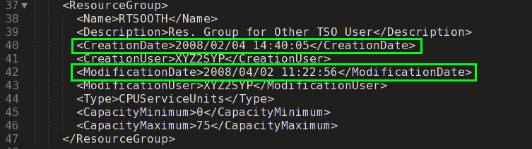
Here is a fragment of a real customer policy, showing a resource group definition:

It’s pretty easy to read. Obviously the XML elements whose node name start with “Creation” or “Modification” are of interest here.

So I modified my PHP code to produce the following two tables:

I’ve tested this with a couple of customers. Basically it counts which years things were created and also modified.

In the real life example there is a gap of a couple of years – a few years ago – but otherwise the story is one of continual maintenance.

In the case of the other test customer it was interesting to hear them translate userids into names; Some of the people were still working for the customer while others had retired. While this might seem like “tourist information” I do believe quite a bit of the job I do is social.

So these two customer cases aren’t huge leaps forward, but it’d be interesting to see what happens when I encounter a customer who hasn’t maintained their WLM policy recently.

There are some issues with this method:

  • The precise items created and updated aren’t reflected in this current report, nor are the precise changes e.g. How a goal’s velocity was altered.
  • The granularity of items changed isn’t great.
  • For an item that has been modified the data only contains the created and last modified date, with no hint of any intermediate changes.

One thing I could fix is producing a more detailed report; For now I have to hunt for the time stamps in the HTML report I produce. So, for example, knowing when a bunch of classification rules were added could be interesting.

As I said at the beginning it was a thought; I’m not convinced there’s a huge amount of value in this but, as with so many new data, evolving code and more experience with real customer situations I might change my mind.[2]


  1. Perhaps I should’ve thought first, and written second. Now, now, settle down. πŸ™‚  β†©

  2. I’m not actually a pessimist but data always looks least useful right at the beginning.  β†©

Reviewing The Situation

(Originally posted 2015-12-14.)

I might have written about this before but it’s such a nebulous subject Web searches don’t enable me to tell. In any case it’s a subject worth reviewing every now and then.

The subject is “when to review your WLM policy”.

I’ve written extensively on how to look at a policy.

While I think you should read Analysing A WLM Policy – Part 1 I want to refer to something I wrote in Analysing A WLM Policy – Part 2.

I talked about 3 categories of WLM policy:

And I noted it was Category 3 that was the most problematic.

I’ve reviewed a fair few WLM policies since then – and I stand by what I said.

But, as is so often the case, applying a “calendar line” view is useful here.[1]

If I were to hatch a rule it would be “all WLM policies evolve to Category 3”.

No policy should remain static, and there are as many cases where the policy should have evolved but didn’t as there are of unhelpful changes.

Two examples:

  • The machine configuration changed but velocity goals weren’t re-evaluated.
  • Response time goals weren’t adjusted to meet the needs of the business.

The evolution towards Category 3 occurs over time, for example as new workloads appear. (And when they disappear clean up seldom happens.)

So, aside from explicit reasons like new hardware, or new applications, I think that someone should take a good look at a WLM policy every few years. Almost inevitably it will have deteriorated in that time.

By the way I don’t care who does the review – so long as they’re competent. While I get to see my fair share of WLM policies, it’s not my prime job. (Though it is a key topic in many customer conversations.) So it’s not my intention to sell you Services.

Talking of “competent”, one thing I like to emphasise is remaining plugged into the (evolving ) folklore. For example conferences, Redbooks, Facebook, Twitter, LinkedIn, user groups like MXG-L and IBM-MAIN, blogs like this (!), etc. Wherever people discuss stuff, in fact.

That way, if it is you reviewing the situation, you stand a good chance of doing a great job. Likewise of knowing when the time has come for such a review.

My main source of information on changes to a customer’s WLM policy is what I get when they send me the WLM ISPF TLIB.[2] I get:

  • Notes – and most customers use the policy notes to log changes.
  • Lots of “created” and “modified” footprints in the sand in the policy itself, complete with the userid of whoever made the change. This leads to interesting discussions sometimes. πŸ™‚

I’d be interested in hearing readers’ views on WLM policy maintenance.

I suspect, for instance, policy changes are often documented more fully in the installation’s Change Management system than in the notes in the policy.

I also suspect most customers are still using the WLM ISPF Application, rather than z/OSMF. I’ve no recommendation to make on this, except to note investment is most likely to be made in z/OSMF.


  1. cause nothing lasts forever, even cold November rain. πŸ™‚  ↩

  2. Generally there’s less breakage if I get a TLIB than XML, the latter usually requiring me to waste time repairing it with a text editor.  ↩

Thanks In Five Languages – ITSO 2015 Tour

(Originally posted 2015-12-10.)

I’ve been very lucky (and kept busy and challenged) these last two months.

In addition to my usual case load of customer situations I’ve had the enormous privilege of participating in the ITSO 2015 Mainframe Topics tour. I’ve presented whole-day sessions on Performance and Availability in five cities: Amsterdam, Paris, Warsaw, Vienna and Bromsgrove.[1]

The main topics have been:

  • Software Pricing and Performance Specialists’ role in it
  • z13
  • zEDC

I’ve learnt an enormous amount, and some of the questions have been really good. Several participants have opened my eyes by sharing experiences.

And I’ve met splendid people – both old friends and new.

I’ve injected some of my experiences, where I hope it’s been useful to.

So this is really a “straight out of my brain onto the page” thank you post to all who participated.

And I hope next year I get to author some slides of my own and take them on tour.


  1. Hence the “five languages”.  ↩

A Note On Velocity

(Originally posted 2015-12-07.)

Not to be confused with Notational Velocity.

A recent customer situation reminded me of how our code calculates velocity. It’s worth sharing with you.

The standard way of calculating velocity is to compute

(Using Samples)/(Using Samples + Delay Samples)

and convert to a percentage by multiplying by 100.[1]

The numbers are all recorded in SMF Type 72 Subtype 3.

We have two main graphs associated with Velocity for a single service class period:

  • How the velocity attained varies with the amount of CPU in the service class period.
  • What the Delay Samples and Using Samples are, by time of day, for the service class period.

You would expect the two graphs to agree – with the Using Samples as a proportion of the whole similar to the velocity data points. Indeed I hadn’t questioned that until this situation.

The surprise was that the Using Samples suggested a far higher velocity than that we computed. In detail, the Using Samples were dominated by Using I/O.[2]

The surprise was only momentary because our reporting also tells us that in this sysplex I/O Priority Management is disabled. This is unusual in my experience and one implication is that neither Using I/O nor Delay For I/O samples are included in the velocity calculation.

So why did my velocity calculation work? It’s because we use two key fields in the SMF 72–3. They are the headline Using (R723CTOU) and Delay (R723CTOT) Sample counts – which reflect how WLM itself calculates velocity. We don’t use the individual Delay an Using sample counts e.g Delay For CPU (R723CCDE) or Using zIIP (R723SUPU) in the velocity calculation.

A few things flow from this:

  • We could produce “With I/O Samples” and “Without I/O Samples” velocity calculations and use them to guide customers in adjusting their goals.
  • We could tally up Using and Delay samples and compare to the headline counts. This way we can see how complex things like zIIP samples play.

But those ideas are for another day or, more likely, another year (it being December now).

But let’s look at a worked (real) example. This is summing over 1 hour for the “DB2STC”[3] service class for 1 system.

The headline sample counts in that hour are:

Category Samples
Using 1101
Delay 1349
Idle 235912
Unknown 28571

If you calculate the velocity it’s about 45%. Also Using + Delay is about 6%, fairly typical for this kind of work, the vast majority being Idle.

Breaking down Using and Delay samples, using the explicit fields in 72–3:

Category Samples
Using CPU 928
Using zIIP 173
Delay CPU 1200
Delay zIIP 144
Delay For Swap In 5

The above doesn’t include Using I/O and Delay for I/O but the samples included do add up to the headline numberss. I’ve also excluded any zero-value counts, including “Using zIIP on CP”.

Now here are the I/O related sample counts:

Category Samples
Using I/O 14715
Delay for I/O 289

If these samples are added in the resulting velocity is 91%. In fact the goal is Importance 1, Velocity 70% – so the goal would be easily met if I/O Priority Management were enabled.

But that doesn’t necessarily mean better performance: Up to a point CPU queuing would be masked by the very strong Using I/O component. But a revised goal of, say, Importance 1 Velocity 90 with I/O in might be better.

Food for thought.


  1. Unknown Samples and Other Samples, while recorded by RMF, are not used in the calculation.  ↩

  2. Delay For I/O Samples were minimal.  ↩

  3. What’s in a name? It turns out this service class provably (from SMF 30, as we always do) contains the MSTR, DIST and DBM1 address spaces for the customer’s Production DB2 on this system.  ↩

Twitter Polls: An Early View

(Originally posted 2015-12-05.)

It’s very early days for Twitter Polls but I think they have promise.

So here’s a post on my experience with them in their infancy. [1] The point of writing about it is twofold:

  • To encourage others to try it – both as a pollster and as a respondent[2].
  • To encourage Twitter to tweak it a bit.

I’m always looking for ways to interact with people. As you probably know Twitter is one of my favorite ways. So it was with some anticipation I learned of Twitter Polls.

Twitter Polls

As a Twitter user you can easily create a poll, with up to 4 choices. Other users have 24 hours to cast their votes – using the Twitter web application. They can vote only once.[3]

After 24 hours the poll is closed and the results published on the pollster’s Twitter page. Both the votes and the % for each option are shown.

A Little Experiment

The only way to form a view about something like this is to try it. So I created a test poll…

This blog is called “Mainframe, Performance, Topics” so asked which of these 3 I should concentrate most on.

It wasn’t a very serious poll, and I made that quite clear. But I have to start somewhere.

20 hours in I had the following votes:

  • Mainframe – 4
  • Performance – 2
  • Topics –2

Not many votes overall – but that’s OK. So I tweeted a chivvy and got 1 more vote. πŸ™‚

The final results were:

  • Mainframe – 4
  • Performance – 2
  • Topics – 3

I found it straightforward to conduct a poll but I have some observations.

And, by the way, the poll wasn’t meant to actually help me decide too much on what to write about. Focus groups aren’t my thing. And I’m not dejected by the low turn out: 9 out of over 2000 followers.

Observations

When you create a poll it’s very easy. But you can’t write much for the poll question, and especially not for the choices. I suspect it’s fitting inside 1 or 2 standard (140 char) tweets, or maybe a 256-minus-protocol-byte block.

More poll “real estate” would be helpful.

And I’d like the choices to include pictures: Suppose I wanted my followers to help pick my blog’s new masthead graphic.

I’ve only seen the poll show up properly in the Twitter web application. Talking to the developers of Tweetbot – usually quick to adopt – they tell me there is no public API for Twitter Polls. I want to add “yet” as clearly that helps make this more pervasive.

More Twitter clients participating means better polls.

Not to insult my pollees but maybe people who use the web application have different views from those that use e.g. mobile clients.

In my poll I’d’ve liked pollees to be able to vote more than once. I suspect they’d’ve liked it, too. Voting more than once might be multiple thumbs up and encouragement. Which takes us on to use cases – in conclusion.

Conclusion

Because you can only vote once you can’t show support for multiple propositions. You might, for example, have wanted to encourage me to write about “Mainframe” and “Performance”. But you can’t. So this instrument is a bit blunt.

So we’re down to “make your mind up” sort of polls. Which I think are still valuable.

I do think Twitter Polls show a lot of promise and I sincerely hope they develop into something that fulfils that promise. Some of the points in “Conclusions” look more resolvable than others. But what do I know? πŸ™‚


  1. Early December, 2015  β†©

  2. I like the term “pollee” but I fear it doesn’t exist.  β†©

  3. It appears the pollster can’t themselves vote.  β†©

A Parked Topic

(Originally posted 2015-11-30.)

In IRD And Hiperdispatch – Wrong ’Em Boyo I briefly mentioned the concepts of Parking and Unparking. It wasn’t appropriate to cover them in depth there. So I’ll talk about them now, focusing on the RMF instrumentation.

But first a brief discussion on Parking versus IRD Logical Processor Management.

  • IRD could – without Hiperdispatch – vary logical processors on and offline.[1] You can observe the behaviour using SMF70ONT in the Logical Processor Data section.[2]

  • Hiperdispatch doesn’t vary logical processors online and offline. SMF70ONT will show each engine online for the whole interval. Instead it parks and unparks them, with a parked engine selecting no work to run.

The data that describes parking is in SMF 70 but not in the Logical Processor Data section. Instead it’s in the CPU Data section.

Why Does What Section It’s In Matter?

It’s because some SMF 70 sections are PR/SM-originated and some related only to this z/OS system. The parking-related data is in a section that is in the latter category.

This means to understand Hiperdispatch parking and Unparking you need to collect SMF 70 data from all significant systems. Our reporting takes data from all systems from which it’s generated, and yours should too.

So What Is This Data?

For parking it’s one field: SMF70PAT, described here:

So, a logical processor that is online but parked will show

  • A full interval’s worth of Online Time in SMF70ONT.
  • A full interval’s worth of Parked Time in SMF70PAT.

If you draw the two data sources together you can make sense of parking, particularly if you understand the Polarization picture (described in IRD And Hiperdispatch – Wrong ’Em Boyo)

And believe me our code in this area has got very complex. πŸ™‚ And it’s going to get more complex soon… πŸ™‚[3]


  1. Early on IRD would vary low-numbered logical processors offline first – which wasn’t great for handling I/O interrupts. Then it changed to the high-numbered processors first.  β†©

  2. Offline Processors Can’t Hurt You might be a useful post to review at this point.  β†©

  3. In fact since drafting this yesterday a couple of nice little tweaks went in. πŸ™‚  β†©

IRD And Hiperdispatch – Wrong’Em Boyo

(Originally posted 2015-11-27.)

Applying the maxim “the customer is always right” this week revealed a bug in my analysis code. It also gave me the opportunity to write about how RMF sees the interaction between IRD Weight Management and Hiperdispatch.[1]

But let me start with some brief, basic information about the technologies in question. If only this proves useful the blog post will still have been worthwhile.

IRD Weight Management Basics

The initial implementation of PR/SM managed LPAR CPU access using static weights.

A long time later Intelligent Resource Director (IRD) introduced three new capabilities, two of which are related to CPU:

  • Weight Management
  • Logical Processor Management

The third, not the topic of this post, is about I/O priority management.

Weight Management introduced Dynamic Weights: Weights could shift between a group of LPARs on a machine, called an “LPAR Cluster”. The total weight for an LPAR Cluster is constant.

Weight shifting occurs in response to WLM’s view of goal attainment.

With Logical Processor Management an LPAR’s logical processors would be varied on and offline. (RMF Field SMF70ONT reflected for how long in an interval the logical processor was online.)

Hiperdispatch Basics

What follows is an extremely basic introduction to one aspect of Hiperdispatch. But it will, I think, suffice.

Without Hiperdispatch an LPAR’s weight is distributed evenly across all its online logical processors – so-called Horizontal CPU Management.

With Hiperdispatch, an LPAR’s weight is distributed unevenly (think “in a focused manner”) across its online logical processors – so-called Vertical CPU Management.

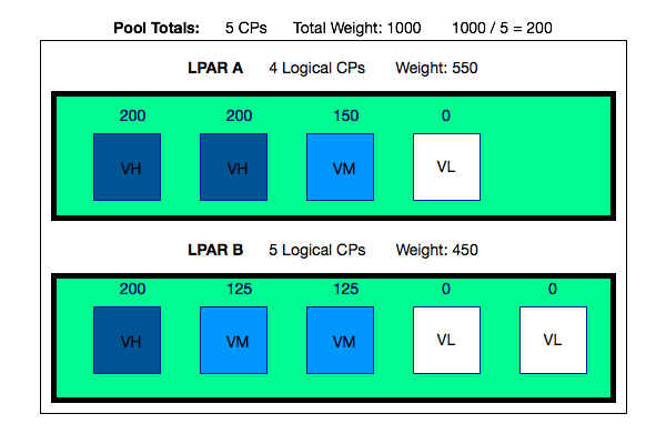
Consider the following (confected and so simpler than in real life) example of a machine’s processor pool. It contains 5 physical processors and the two LPARs’ weights add up to 1000.

So a physical processor’s weight’s worth is 1000 / 5 or 200. Hang on to the 200 as it’s important in what follows.

  • LPAR A has a total weight of 550 and 4 logical CPs. Rather than distribute the weight across all 4, a pair of CPs are designated Vertical High (VH) and assigned a weight of 200 each. The remaining 150 goes to a third CP, which is designated a Vertical Medium (VM). The fourth logical CP has a weight of 0 and is deemed a Vertical Low (VL). It can be “Parked”, meaning work is prevented from running there. It can also be “Unparked” and then work can run there.

  • LPAR B has a total weight of 450 and 5 logical CPs. It has 1 Vertical High, leaving a further 250 in weights to distribute. But rather than having 2 Vertical Highs and a Vertical Medium with (a rather puny) weight of 50 Hiperdispatch splits this remaining 250 across 2 Vertical Mediums, each with a weight of 125. The remaining logical CPs are, of course, 2 Vertical Lows with weights of 0.
It’s beyond the scope of this post to describe how logical processors map onto physical processors, except to say the Vertical Highs are pseudo-dedicated.

One thing to note is with Hiperdispatch enabled Logical CPU Management is no longer available. Hiperdispatch’s Parking and Unparking mechanism does a rather more sophisticated version of what Logical CPU Management did.

But the above example is a static picture.

Hiperdispatch Interaction With IRD Weight Management

With IRD Weight Management it’s possible [2] for the LPAR weights to shift. Taking the previous example and further supposing the two LPARs are in an LPAR Cluster…

Suppose the weights shift by 50 in favour of LPAR A. So LPAR A’s new weight is 600 and LPAR B’s is now 400.

The picture is now as follows:

You’ll notice the Vertical Polarization is now different:

  • LPAR A now has 3 Vertical Highs, rather than 2 Vertical Highs and 1 Vertical Medium. It still has 1 Vertical Low.
  • LPAR B now has 2 Vertical Highs, rather than 1 Vertical High and 2 Vertical Mediums. The number of Vertical Lows is increased from 2 to 3.

Notice the number of logical processors assigned to each LPAR hasn’t changed, only the share of the processor pool (or the weights).

My Bug

My code said a specific LPAR had 7 General Purpose engines (GCPs) but the customer said it had 8.[3] And those were genuinely the numbers.

The customer, as I hinted, was right.

So let me explain now how RMF instruments all this (well a little of it ). SMF70POF is a field in the Logical Processor Data Section, of which there is one per logical processor for every LPAR (as described in Offline Processors Can’t Hurt You).

Here is an extract from the SMF manual:

  • Bits 0 and 1 indicated whether and how the processor is polarized .
  • Bit 2 indicates this changed during the interval.

Combinations of these bits do the job of telling me the story of the logical processor’s polarization through the RMF interval.

In a nutshell what happened was my code didn’t count processors that transitioned in the period of interest from e.g. Vertical High to e.g. Vertical Medium. It certainly counted processors in 6 categories:

  • Unpolarized (or rather Horizontally Polarized )
  • Vertical High
  • Vertical Medium
  • Vertical Low
  • Vertical Transitioned
  • Unknown

The code was meant to add up all totals but 1 was missing. And IRD shifting weights caused, for once, a processor to appear in the Vertical Transitioned category.

Anyhow the bug is fixed now and one of the results is this post. So I guess that’s progress. πŸ™‚ And I’m genuinely grateful to the customer for spotting the error, even if it cost an hour or so of heartache.


  1. I talk quite a bit in the current ITSO 1-day workshop on Performance and Availability. (These are not my slides .)  ↩

  2. In practice, in many customer sets of data the weights don’t shift, but for a substantial minority they do. Not dramatically, but they change.  ↩

  3. A bit like The Clash’s Wrong ’Em Boyo (from the excellent London Calling): “Stagger Lee throwed seven / Billy said that he throwed eight” – hence part of the title of this post. A gratuitous reference if ever there was one. πŸ™‚ />  ↩

(Originally posted 2015-11-27.)

Applying the maxim “the customer is always right” this week revealed a bug in my analysis code. It also gave me the opportunity to write about how RMF sees the interaction between IRD Weight Management and Hiperdispatch.[1]

But let me start with some brief, basic information about the technologies in question. If only this proves useful the blog post will still have been worthwhile.

IRD Weight Management Basics

The initial implementation of PR/SM managed LPAR CPU access using static weights.

A long time later Intelligent Resource Director (IRD) introduced three new capabilities, two of which are related to CPU:

  • Weight Management
  • Logical Processor Management

The third, not the topic of this post, is about I/O priority management.

Weight Management introduced Dynamic Weights: Weights could shift between a group of LPARs on a machine, called an “LPAR Cluster”. The total weight for an LPAR Cluster is constant.

Weight shifting occurs in response to WLM’s view of goal attainment.

With Logical Processor Management an LPAR’s logical processors would be varied on and offline. (RMF Field SMF70ONT reflected for how long in an interval the logical processor was online.)

Hiperdispatch Basics

What follows is an extremely basic introduction to one aspect of Hiperdispatch. But it will, I think, suffice.

Without Hiperdispatch an LPAR’s weight is distributed evenly across all its online logical processors – so-called Horizontal CPU Management.

With Hiperdispatch, an LPAR’s weight is distributed unevenly (think “in a focused manner”) across its online logical processors – so-called Vertical CPU Management.

Consider the following (confected and so simpler than in real life) example of a machine’s processor pool. It contains 5 physical processors and the two LPARs’ weights add up to 1000.

So a physical processor’s weight’s worth is 1000 / 5 or 200. Hang on to the 200 as it’s important in what follows.

  • LPAR A has a total weight of 550 and 4 logical CPs. Rather than distribute the weight across all 4, a pair of CPs are designated Vertical High (VH) and assigned a weight of 200 each. The remaining 150 goes to a third CP, which is designated a Vertical Medium (VM). The fourth logical CP has a weight of 0 and is deemed a Vertical Low (VL). It can be “Parked”, meaning work is prevented from running there. It can also be “Unparked” and then work can run there.

  • LPAR B has a total weight of 450 and 5 logical CPs. It has 1 Vertical High, leaving a further 250 in weights to distribute. But rather than having 2 Vertical Highs and a Vertical Medium with (a rather puny) weight of 50 Hiperdispatch splits this remaining 250 across 2 Vertical Mediums, each with a weight of 125. The remaining logical CPs are, of course, 2 Vertical Lows with weights of 0.

Hiperdispatch Before IRD Weight Shift

It’s beyond the scope of this post to describe how logical processors map onto physical processors, except to say the Vertical Highs are pseudo-dedicated.

One thing to note is with Hiperdispatch enabled Logical CPU Management is no longer available. Hiperdispatch’s Parking and Unparking mechanism does a rather more sophisticated version of what Logical CPU Management did.

But the above example is a static picture.

Hiperdispatch Interaction With IRD Weight Management

With IRD Weight Management it’s possible [2] for the LPAR weights to shift. Taking the previous example and further supposing the two LPARs are in an LPAR Cluster…

Suppose the weights shift by 50 in favour of LPAR A. So LPAR A’s new weight is 600 and LPAR B’s is now 400.

The picture is now as follows:

Hiperdispatch After IRD Weight Shift

You’ll notice the Vertical Polarization is now different:

  • LPAR A now has 3 Vertical Highs, rather than 2 Vertical Highs and 1 Vertical Medium. It still has 1 Vertical Low.
  • LPAR B now has 2 Vertical Highs, rather than 1 Vertical High and 2 Vertical Mediums. The number of Vertical Lows is increased from 2 to 3.

Notice the number of logical processors assigned to each LPAR hasn’t changed, only the share of the processor pool (or the weights).

My Bug

My code said a specific LPAR had 7 General Purpose engines (GCPs) but the customer said it had 8.[3] And those were genuinely the numbers.

The customer, as I hinted, was right.

So let me explain now how RMF instruments all this (well a little of it ). SMF70POF is a field in the Logical Processor Data Section, of which there is one per logical processor for every LPAR (as described in Offline Processors Can’t Hurt You).

Here is an extract from the SMF manual:

SMF70POF

  • Bits 0 and 1 indicated whether and how the processor is polarized .
  • Bit 2 indicates this changed during the interval.

Combinations of these bits do the job of telling me the story of the logical processor’s polarization through the RMF interval.

In a nutshell what happened was my code didn’t count processors that transitioned in the period of interest from e.g. Vertical High to e.g. Vertical Medium. It certainly counted processors in 6 categories:

  • Unpolarized (or rather Horizontally Polarized )
  • Vertical High
  • Vertical Medium
  • Vertical Low
  • Vertical Transitioned
  • Unknown

The code was meant to add up all totals but 1 was missing. And IRD shifting weights caused, for once, a processor to appear in the Vertical Transitioned category.

Anyhow the bug is fixed now and one of the results is this post. So I guess that’s progress. πŸ™‚ And I’m genuinely grateful to the customer for spotting the error, even if it cost an hour or so of heartache.

  1. I talk quite a bit in the current ITSO 1-day workshop on Performance and Availability. (These are not my slides .)  ↩

  2. In practice, in many customer sets of data the weights don’t shift, but for a substantial minority they do. Not dramatically, but they change.  ↩

  3. A bit like The Clash’s Wrong ’Em Boyo (from the excellent London Calling): “Stagger Lee throwed seven / Billy said that he throwed eight” – hence part of the title of this post. A gratuitous reference if ever there was one. πŸ™‚  ↩

A Picture Of Dedication

(Originally posted 2015-11-22.)

Sometimes a little visual tweak can make all the difference. This post is about one such case.

Actually the code change to achieve it was quite complex but the visual rearrangement is simple.

I have a number of customers with Integrated Coupling Facility (ICF) processor pools with both dedicated and shared Coupling Facility (CF) processors.

For Production most people (sensibly) define their ICF LPARs with dedicated processors. But it’s perfectly legitimate for Test or Development Parallel Sysplexes to use shared processors.

Both the customers whose data I’m looking at right now have such a mixed arrangement. [1]

Existing Depiction

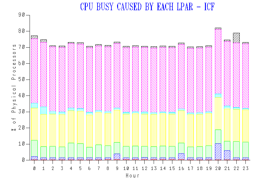
Up until now our code has stacked up ICF LPAR CPU usage by time of day like so:

Though you can’t see it (as I’ve cropped the legend off) the LPARs are stacked alphabetically. There’s been no more logic to it than that.

The purple and yellow LPARs turn out to have 2 dedicated processors and 1 dedicated processor, respectively. While you probably could tell that, it’s really not “in your face”.

New Depiction

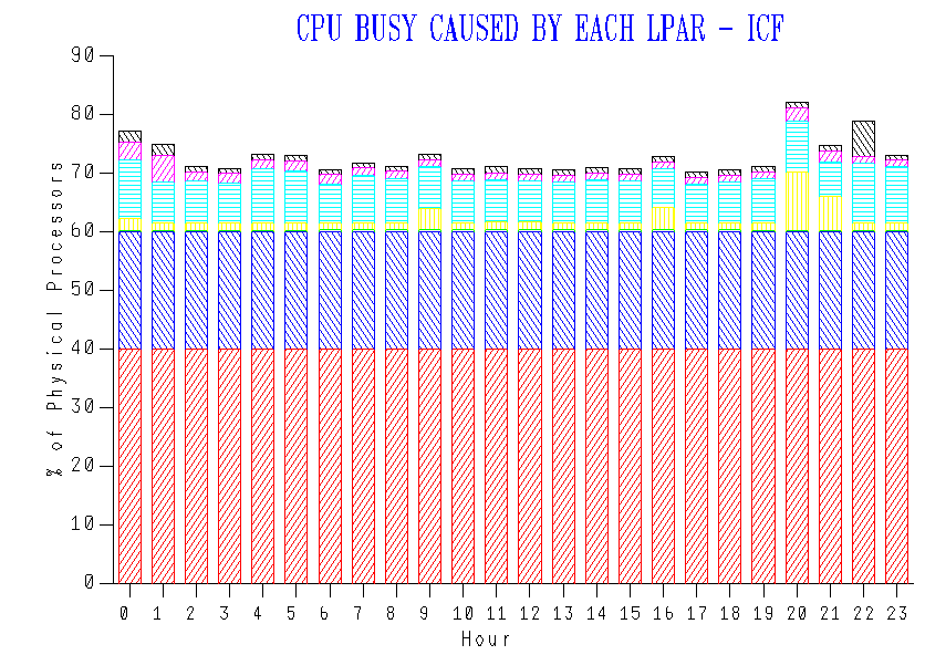
Consider the following redrawing: [2]

In this redrawing I sorted the LPARs by Number Of Dedicated Processors descending and, within that, alphabetically.

Here we clearly have two LPARs with dedicated processors. This being the ICF pool the ICF LPARs don’t give the processors back.

The remaining LPARs share what’s left of the pool.

You can see the red LPAR uses 40% of the pool and the blue one 20%. We happen to know that the pool has 3 dedicated ICF processors and 2 shared.

We’re much more clearly depicting the 2 LPARs with dedicated processors.

As I said this is a minor tweak, but it’s a much nicer result. If you’re graphing your ICF processor pool you might like to consider this rearrangement of stacking.

There are some further tweaks I could make. For example:

  • I could make the y axis the number of processors and make it end at (in this case) 5 processors.
  • I could make the series labels show e.g. “2 ded” for an LPAR with 2 dedicated processors.

At the beginning I said the code change was substantial, though the visual change was small. I now have much more control over the construction of this graph, so I can do things with axes I couldn’t before. Similarly I can do things with series labels I couldn’t before.

I mention this re-engineering as I half expect it to enable more creativity in how we depict processor pools. If anything worthy of sharing comes up I’ll share it here. Stay tuned!


  1. I suspect the third customer, whose data is just arriving, will turn out to be the same.  ↩

  2. And ignore the colour changes.  ↩

Good Things Come in Threes?

(Originally posted 2015-11-16.)

It's that time of year when I start to think about writing conference presentations for user groups and conferences in 2016.

Already I have three in mind, with varying degrees of sketchiness. Their working titles are:

  • He Picks On CICS
  • Fun With DDF
  • So You Want To Be A Better Performance Specialist?

I don't want to “design by committee ” and as for focus groups yeugh! πŸ™‚ But I do care about what what topics my readers and audience are interested in.

I have my ideas, as the above list shows, but I'd like to hear yours.

IBM doesn't mind what I write about, there being no agenda other than the obvious one of “mainframe performance is fascinating”. Presentations are another matter as I really need a platform – whether a conference or a user group.1

It's not an “either or” situation: I could produce a barrage of presentations for the conference season2, or dribble them out throughout the year.

I'm experimenting with Twitter Polls 3 so I might do one on this list of topics. The relative shares will be interesting but more so the level of interest. My Twitter following, though, is dominated by people who aren't mainframers.

Worth a try once, though, as so many things are. πŸ™‚

(This post was banged out on my phone between Heathrow and Munich, en route to speaking all day at an ITSO workshop in Warsaw.)


  1. Actually that's not strictly true as good material comes in handy at unexpected times. And there's always Slideshare. And besides I learn quite a bit by writing. 

  2. I'm not entirely sure when this is: Formally it could be System z Technical University in May, but user group meetings happen all the way through the year. 

  3. It appears Twitter are only experimenting with this as well right now: There is no API, Tweetbot tell me. Furthermore even the web implementation looks basic, with very short choice text limits. 

Captivating Capture Ratios

(Originally posted 2015-11-15.)

I don’t think I’ve written about the concept of Capture Ratio[1] before. To be honest it’s kind of a “nerdy” or “internal” thing. But a recent experience suggests to me it is interesting, even if only for the wrong reason.

What Is Capture Ratio?

Not all CPU in a z/OS system can be attributed to a service class: If you add up all the CPU in SMF 72–3 (Workload Activity) it always amounts to less than the CPU in SMF 70–1 (System-Level).

If we divide Workload CPU by System CPU and turn it into a % we get a Capture Ratio. [2]

So what do we expect? Our observations are

  • Generally most systems show capture ratios in the range 85% to 95%.
  • Capture ratios vary, but not usually by very much. [3]
  • Capture ratios are lower for very low utilisation systems than very high utilisation ones.
  • Capture ratios are lower for highly paging systems, and probably for high I/O ones.

Generally I don’t see anything better about a system with a capture ratio in the low 90’s than one in the high 80’s, percentagewise. So I wouldn’t fret about that.

How Do We Use Capture Ratio?

As I indicated at the outset, this has been an internal thing.

In a recent study, to tweak nobody’s nose at all, we saw appallingly low and more or less random capture ratios. It turned out we were missing lots of 72–3 records.[4] So the capture ratio was a good diagnostic tool.

Despite what I said about capture ratio being “internal” we have a standard chart that plots capture ratio for a system by day. This is why I know about the behaviours listed above.

What Went Wrong?

In some studies over the past few years our capture ratio has gone over 100%. It really shouldn’t.

While this has been “subliminally troubling” it hasn’t been enough to make me spring into action. With a recent study, however, we were getting capture ratios of hundreds of percent. Enough to set alarm bells ringing. So Dave Betten and I set to debugging.

It’s all down to zIIP: We only get capture ratios above 100% when both the following are true:

  • We have substantial zIIP CPU relative to GCP CPU.
  • The zIIP Normalisation Factor is substantially higher than 1.

Our code has a combined capture ratio, plus separate ones for GCP and zIIP CPU. We plot the former but have ignored the latter two.

I saw the pattern: Excessive zIIP capture ratio. Dave debugged the logic, which confirmed it. We’re using the zIIP Normalisation Factor[5] wrong in both the general and zIIP capture ratio calculations.

Adjusting the zIIP capture ratio in a spreadsheet one system’s pair of capture ratios look like this:

I’ve summarised across 8-hour shifts and the x axis is a shift number.

The numbers appear to have “come right” and examining our logic suggests they should be right.

I think I discern that most of the time zIIP capture ratio is slightly above GCP capture ratio. This is what I’d guess, based on zIIPs not doing I/O. But I’m not 100% sure. Future data sets will tell.

Interestingly, the “wrong calculation” zIIP capture ratio was proportionately worse for a system on a machine where the zIIP Normalisation Factor is 6.22 than the ones where it is 2.36. But that’s not surprising.

Putting It Right

One key lesson is: Don’t boost everything by capture ratio to fill in gaps.

  • The “low and random” case shows that’s not good idea as you introduce distortion that way.
  • The “impossibly high” case shows something fundamental is wrong.

So we know what the “excessively high” case is caused by. Now to get a fix tested and into Production.

And you might expect to see (at least pedagogically) a new chart that separates zIIP Capture Ratio from GCP Capture Ratio. I think this “fine structure” will be useful to glean.

So I hope I’ve shown that Capture Ratio is interesting, even without the bug we’ve troubleshot.

And “every day for us something new, open mind for a different view, and nothing else matters” [6] applies to this. Comme d’habitude. πŸ™‚


  1. I’ve seen people write “capture ration” and it’s not been people for whom English isn’t their first language, but it could be autocorrect. πŸ™‚  ↩

  2. Of course this is technically wrong as it’s a percent, not a ratio. Nevermind. πŸ™‚  ↩

  3. This stability is fairly reassuring. It seems like a real thing.  ↩

  4. This has now been resolved and we have complete set of 72–3 data.  ↩

  5. You have to divide what’s in SMF 70–1 and in SMF 72–3 by 256 – which implies a granularity all of its own.  ↩

  6. Nothing Else Matters  ↩