(Originally posted 2018-07-28.)

It’s the Time Of The Season¹ for thinking about Day One support. Not for z/OS, or DB2, or CICS, or anything mainframe-related. But for iOS, MacOS and their kin.

Before you switch off – if you’re an Android user² – you can consider the Apple bit an analogue. This post will be light on technical detail, and heavier on developers’ approaches. It might even stimulate some discussion about z/OS.

So, it’s a month or so since Apple announced new iOS, MacOS, etc releases at their Worldwide Developer Conference (WWDC) and developers (and foolish / brave non-developers) have run betas. Several betas, in fact.

Part of the point is to prepare their products for General Availability³. And developers’ approaches to that is what this post is about.

So, you can see this might have some relevance to z/OS and its vendor ecosystem.

Approaches To Day One

As I look around at the many iOS, WatchOS, and MacOS apps I have I see a number of approaches from the various developers. Here are a few examples:

• I’m beta’ing releases of Drafts (mentioned in Appening 5 – Drafts On iOS). Already the sole developer is experimentally introducing exploitation of the new Siri Shortcuts feature.
• I use a podcast client called Overcast. The sole developer – Marco Arment – is rebuilding his WatchOS app to use the new iOS 5 audio playback capabilities.
• I’ve yet to hear much from the Omni Group but they indicated they were clearing the decks for whatever Apple threw at them – which is a good sign.
• I’m hearing rumblings that some of the MacOS apps I depend on – some IBM, some not – won’t Day One support the new Mojave MacOS release.
• There are plenty of apps on my iOS devices that already won’t run – because the developer never updated them to run on iOS 11. The technical point here is they must be 64-Bit. I consider these – 1 year in – as “abandonware” though I wish Apple did a better job of enabling me to dispose of them.

Through these various approaches and stances runs a theme: I’ve emphasized the words “sole” and “Group” for a reason.

• The sole developers, Greg and Marco, are moving fast and experimenting with exploitation.
• Casting no aspersions whatsoever, I see Omnigroup saying little. But I am jolly sure they are working on stuff for the apps I rely on: Omnifocus and OmniGraffle (and the others of theirs I’m not so reliant on). I’m confident for two reasons: Attitude and Track Record.

In Enterprise we might well appreciate the “more planned” approach Omni Group are taking. In the consumer space not quite so much.

But, back in 2014, I wrote in And Just Complain:

Mobile users, though, have no real understanding of how the service is provided and don’t really care (and nor should they.) So I think they can be characterised as much less patient and much less tolerant of service issues, and that’s fine.

So, assumptions of tolerance of errors and issues is in limited supply everywhere.

What Do You Need?

There’s obviously a lot of Marketing value to being able to claim “Day One” support – for some markets. So, from a developer’s point of view, something close to Day One support is important. In “real world” terms there’s another point for developers: They really don’t want to field “iOS 12⁴ broke your app” issues.

For the vendor – Apple or IBM – it’s great to have customers able to adopt their new release on Day One. In reality, though, many customers will want to skip early life and the “pioneer cost” issues⁵ that brings.

A few days ago (as I write this) was World Emoji Day. The relevance of World Emoji Day is surprisingly high: Each year on this day the Emoji standards body releases the new emoji for the year⁶. Apple traditionally supports these on the first point release after a new version of iOS or MacOS. That’s also where the first batch of “settling in” fixes are delivered for an iOS version. It might seem superficial but getting people to install this point release is a lot easier if there are new emoji to play with.⁷

And what about us, hapless punters that we are? 🙂 Some of us are insanely 🙂 keen to install the new operating system level on the day of release. I’m not consistently 🙂 one of those. But pretty close.

When I review the myriad material coming out of WWDC, I take note of the new things⁸. But I consider what the operating system vendor ships as being “one shoe dropping”. I’m really looking forward to the other shoe dropping: What the app vendors ship.

But, of course, z/OS is different, or rather its customers are. Very few will install a new z/OS release at GA, for example. But they would like to know that all their products – whether vendor or IBM – work well before they need them to.

Exploitation might well be a different thing; My suspicion is most customers are less worried about exploitation. Though, if you ask them, quite a few customers will reply “I’m really looking forward to x”.

There is a whole interesting side conversation to be had about what drives customers to upgrade, quite apart from exploitation. Maybe another time. But, even if you’re just upgrading because you have to, it’s still important to know stuff continues to work. If you are a “Last Day Upgrader” (to coin a phrase) the chances are that vendor and IBM products will have introduced toleration.

But I still get excited at reading announcement material and learning about new functions.

(Originally posted 2018-07-26.)

“Mum!” came the cry in the middle of the night. You can imagine how well that was received.¹

“There’s a frog in the bathroom!” shouted my daughter. Indignant or horrified, you decide. 🙂

So, a number of thoughts occurred:

• It can’t do us any harm; It’s tiny and probably more scared of us than any of us are of it.
• Picking it up is not an option; It could be poisonous to touch and probably wouldn’t stay on the plastic safety briefing, even if we got it onto it.
• The lizard we saw in the afternoon in the room escaped as soon as we opened the door. Frogs are at least as smart as lizards… 🙂
• We’re probably not going to tread on it – unless we’re colossally clumsy or stupid.
• Shampoo and shower gel are probably not good for a frog, but otherwise I don’t mind sharing the shower with it. 🙂

Also uttered was “Mum! Why did you let the frog in?” 🙂

Of course the frog was gone² in the morning.

Meanwhile, as I write this on the balcony of our room, there’s a wallaby a few feet below us, foraging³; It knows we’re here but it really doesn’t care. Respect!

(Originally posted 2018-07-09.)

Writing about writing; How meta is that? 🙂

It’s been 4 years since I wrote Appening 3 – Editorial on iOS. (In the same year I went on to write Appening 4 – SwiftKey on iOS. So here we are with another thrilling “Appening” episode.)

Seriously, it’s been a while since I wrote about writing tools. And much has changed since then. But I’ll net it out: I’ve moved most of my writing from Editorial to Drafts – when on iOS.

Sorry, It’s Time To Go

Editorial, if you recall, was a Markdown authoring app with built in workflows. Most particularly, it was extensible through Python. I say “was”. Technically the word should be “is”. But I have my doubts about that, the app not having been updated for years. And that has made most users of Editorial quite nervous.¹

I have to say that I hadn’t invested much time in building workflows in Editorial, but I had become very comfortable with it as a writing tool. One thing that really helped was direct support for Dropbox. What this allowed me to do was to write stuff on either an iPhone or iPad and have it sync to my Mac. And, though I’m not big on pictures in my posts, it could retrieve images from Dropbox when previewing.

For some time now I’ve been writing on iOS devices and finishing off and publishing using Sublime Text. First it was on Linux but, when I got my work Mac in March 2017, I continued using Sublime Text. (Sublime Text has built-in Markdown support and can readily convert to HTML. I paste HTML into this blog site to post.)

Making The Change

I’m now using a nice writing app – Drafts – on iOS. Recently Version 5 was released, which is a rewrite and has a significant set of enhancements over prior versions.

Because I want to support the author and, naturally, I want all the functions² I’ve gone Premium, paying a subscription. I don’t consider it a lot of money and I’m quite careful about how many apps and similar I sponsor. This one is worth it.

One consequence is I’m switching to JavaScript automation from Python. Funnily enough, I now know far more Python than I did then. JavaScript is, of course, almost universal. And, me being me, I have a working knowledge of both³.

There are quite a few workflows available for Drafts, some written in JavaScript and some using composable building blocks. In that way it’s similar to Editorial. One I’ve used in this very post is one that makes footnote creation a snap⁴.

Another one is Markdown Preview – which uses a HTML Preview built in stage. What’s nice about this is it uses an HTML template I can modify. This, as any Drafts workflow could, has placeholders for e.g. the first line of text. Which I think is rather nice.

If you were considering using Drafts as a writing tool you should be aware of one limitation. Recall the bit about Editorial embedding images when previewing Markdown? I haven’t found a way of making Drafts do that. As I finish off writing in Sublime Text – and my images will make it to the Mac anyway – this is only a minor annoyance for me. But if you were doing everything on iOS it might put you off.

Data Input Everywhere

Drafts for many is a “first capture” app for text. The expectation being that you move the text elsewhere. What might be debatable is how late in the text curation process you move it (if at all).

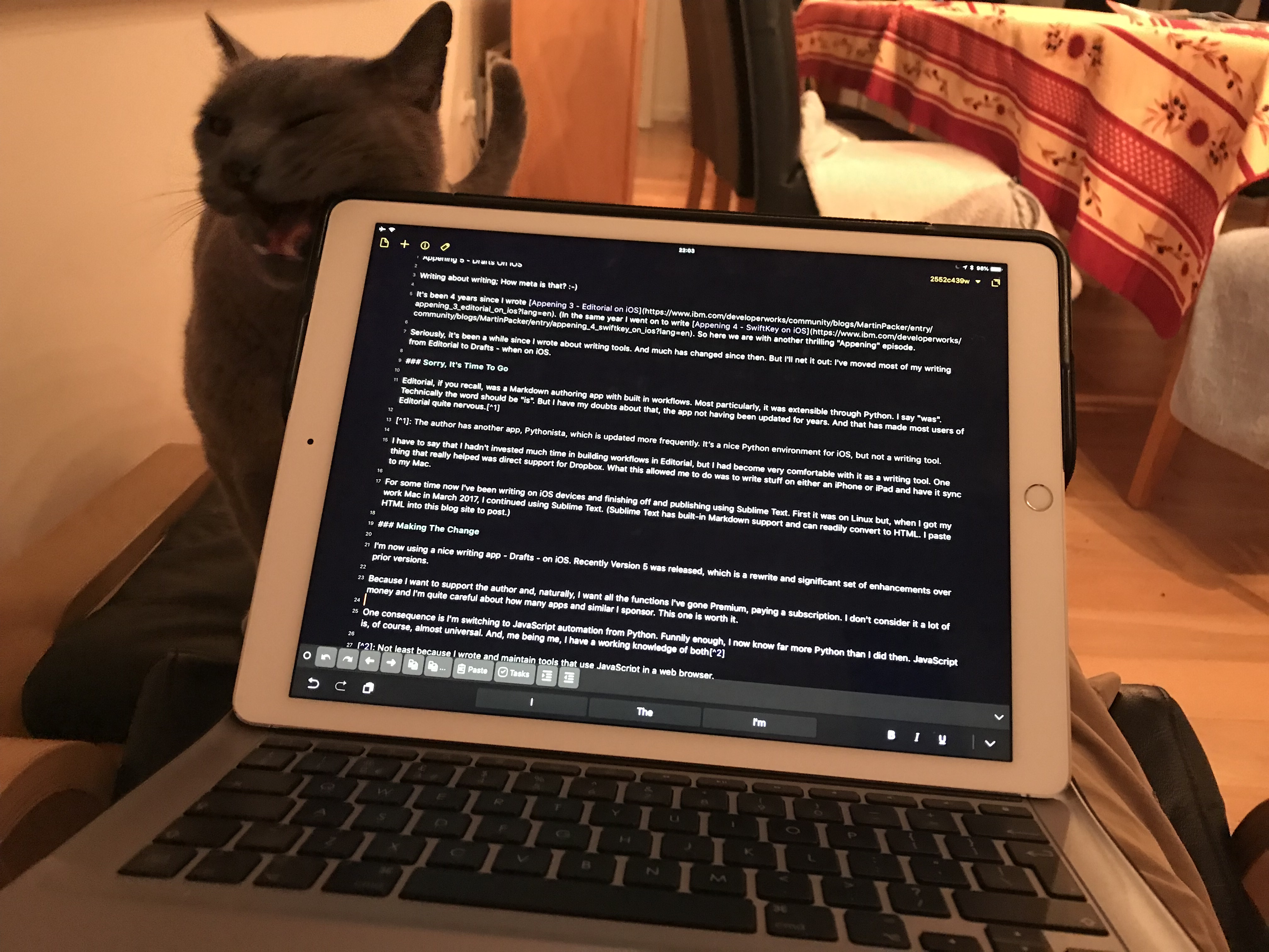
I’m writing this in Drafts right now, using an iPad with an external keyboard. I don’t intend to move it until I’m more or less done with it. I can, through its syncing, continue to edit it on my iPhone. In fact I’ve done that on previous blog posts.

As you can see, sometimes I get some “help” with my writing. 🙂

One of the nice features is that I can capture text by dictating into my Apple Watch. I wouldn’t use that for more than a sentence or two, though. Once dictated, it syncs to Drafts on the iPhone and hence to the iPad.

Actually, through the wonders of the Workflow app (soon to be Shortcuts in iOS12) and x-callback-url inter-app linkage, I can get text into Drafts a number of different ways.

I just like the idea I can get text into it any number of different ways.

Parting Thoughts About Writing

Sometimes my posts start with a title (usually with a bad pun in it). Sometimes they start with a one line notion. At one point I thought that if that was all the payload I shouldn’t bother writing posts but should just tweet. That was 10 years ago and I now know I have rather more to say. In fact I do both; You might’ve noticed that one-liners in tweets turn into pieces of posts.

Anyway, the point is “just get writing, no matter how garbage you think it will be” seems like a reasonable mantra. And I think I need to deliver that to my mentees, as they have points of view to get out.

The other point, and this is what this post is really about, would be this: Be prepared to shake up your writing tools every so often, as new possibilities open up. Particularly ones that mean you can capture ideas anywhere. Technically, that could even be in the bath, with the advent of waterproof phones. 🙂

Most of all, have fun with writing! Now get on with it. 🙂

(Originally posted 2018-07-07.)

Sometimes I can plan ahead, designing analysis code for an upcoming feature of e.g. z/OS. Often, however, a condition falls into my lap – without my having thought about it first. This is about the latter.

It’s about CICS’ support of Java Liberty Profile – or “Lib Profile” for short.

I want to talk about two things:

1. How to detect a CICS region is running the Lib Profile – without using CICS instrumentation.
2. What else you might see from non-CICS instrumentation when that is the case.

I discovered, inadvertently, that a recent customer’s 4 Production LPARs each had a pair of CICS regions running Lib Profile. These happen to be small regions right now, so their performance numbers are small. But, that’s enough to get me sensitised to the topic of this post.

What Is CICS Liberty Profile?

Real CICS people, get your cringing / sniggering over now. 🙂 But do feel free to “well actually”¹ me.

Let’s divide this into two questions:

1. What is Liberty Profile?
2. How does this apply to CICS?

Liberty Profile

WebSphere Application Server (WAS) V8.5 introduced Lib Profile – enabling lightweight java servers, with a quick startup time and a small footprint. It also has configurability – through its (XML) server configuration.

There’s also a strong standards-based flavour to it, through OSGi².

It has less function than the full-function WAS java profile, though selectability (through server.xml) allows you to add from a bunch of functions.

But Lib Profile is not just about WAS. In z/OS 2.1, z/OSMF was reworked to use Lib Profile. So this makes z/OSMF much more consumable – as its footprint and startup times are improved.

CICS Support For Liberty Profile

CICS support for Lib Profile was introduced in 5.1 and enhanced thereafter. Basically you can run Lib Profile applications in a CICS region.

If you want a deeper treatment read the IBM CICS and Liberty: What You Need To Know Redbook.

One thing I note is this Redbook mentions setup considerations for both Type 2 and Type 4 JDBC drivers. To state the obvious the “J” stands for “java”. I’ll mention DB2 in a bit.

Detecting CICS Regions With Liberty Profile

So, I got SMF 30 Interval data from a customer. As loyal readers³ will know, I use the Usage Data Section data to discern what I can about individual address spaces. Mostly this is software level and topology information. More on both of these presently.

My code, for quite a few years now, has detected CICS regions. In this customer there were many and the “DFHSIP” Usage Data Section says CICS TS 5.3. It also mentions DB2 and MQ. So far so good.

I wrote the code in an “open minded” way – so any usage data will show up, including that from some other vendors.⁴

Now, this is where it got interesting. Of the many CICS regions, 8 showed a ‘CICS LIBERTY’ data section. 2 on each of their 4 cloned⁵ LPARs.

This customer has a good CICS naming convention – and these 8 regions followed that, with the LPAR letter embedded in the region name. In this case all 8 regions’ names ended with “J”. Might be the beginnings of an evolution of the naming convention, but I digress.

The point is, the presence of ‘CICS LIBERTY’ in a Usage Data Section tells you the region is using Lib Profile.

Other Numbers You Can See

In many ways these regions are just normal CICS regions. So, I would expect connections to DB2 and MQ to show up in their own Usage Data Sections. Indeed the above-mentioned Redbook makes the point you have to set up the standard CICS/DB2 and CICS/MQ machinery first.

And I do see MQ and DB2 connections for these regions, complete with their versions and subsystem names.

As these are small, I gather under development, regions I’m not surprised the numbers are small. So, the zIIP-eligible CPU for each region is about 0.3% of a processor. The non-zIIP portion is about 0.1%. Like I said, small regions.

So, I would expect that 3:1 zIIP:GCP ratio to be about right, scaled up. But I’m guessing. Recall JNI code and the like wouldn’t be zIIP-eligible. But the application code ought to be. But at least this is readily measurable.

Another thing that is measurable is ZFS / HFS I/O, Pipe I/O etc – as detailed here.

In these regions I only see a relatively small amount of file system I/O. I would expect to see quite a bit more for busier regions. The EXCP counts are modest, too.

Virtual Storage

Virtual storage is an interesting one. You can see allocated virtual storage in the three obvious areas:

• 24-bit (below the line)
• 31-bit (below the bar)
• 64-bit (above the bar)

It’s uncommon these days to see signs of constraint below the bar but the other two warrant some attention. But recall this is allocated virtual memory. There’s nothing in SMF 30 to document how it’s actually used.

For CICS, I would view 31- and 64-bit memory differently.

• For 31-bit I’d be concerned about running out of it.
• For 64-bit I’d just be interested in how much exploitation.

Of course, virtual memory accessed turns into real memory used – at least to a first approximation.

So let’s look at one of these regions, from the virtual storage point of view.

• These regions tend to be close to the 31-bit limit of 1477MB. But I would just say that reflects allocations, not suballocations. I’d want to have some CICS statistics to really nail that.
• The 64-bit usage is about 1.5GB apiece. This reflects a sizeable heap and also the fact this is a 64-bit JVM. By the way the MEMLIMIT is 64GB, set by JCL.

By the way, other writings of mine on the subject of virtual storage include How I Look At Virtual Storage and, from 2004, DB2 Virtual Storage – The Journey Continues.

Conclusion

I’m going to repeat something I’ve often said: The beauty of SMF 30 is that it is scalable. Meaning that you can work with arbitrarily large numbers of address spaces, from many systems. In other words your entire z/OS estate. Something which isn’t true of middleware-specific instrumentation. Few people object to sending me SMF 30; Most are wary of sending middleware-specific SMF across the board.

The aim of this post is to show, yet again, how you can use SMF 30 to scan your CICS regions, bringing the relevant ones to life – at least a little bit.

One thing I’d like to see – and I don’t know how feasible this is – is an encoding of Lib Profile level in the Usage Data Section. Today there is no real clue – with the product number being “0000-000”. But then mangling e.g. ‘16.0.0.3’ into 8 characters might be difficult. Actually that’s an easy one… 🙂

(Originally posted 2018-06-25.)

This post follows on from something I mentioned in When Reality Bytes. Some things I get to immediately; Others take a little time. This is one of the latter.

A more systematic, better, way for classifying work as Mobile was introduced with APARs OA47072 for WLM and OA48466 for RMF in December 2015.

Some months ago I mapped the SMF record improvements OA48466 brought. But I had no data to test the mapping with. Very recently, however, I had the opportunity to develop reporting to go with it. (A recent engagement had a strong Mobile component.) Often a few records are enough to test mappings with. But to begin to develop reporting takes “real world” data. Such is the process.

Mobile Work Classification With OA48466

As I mentioned in When Reality Bytes a new WLM construct was introduced: Reporting Attribute. To classify work as Mobile you simply scroll to the right (enough times) and type in MOBILE in the Reporting Attribute field.¹

Of course, planning and getting to that stage takes some doing. But it’s a lot better than previous schemes involving detailed transaction (SMF 110 CICS Monitor Trace, for instance) reporting. Or dedicated Mobile regions or even LPARs.²

And ensuring your application folks, or whoever, identify to you a workload as Mobile, remains an organisational challenge.

System-Level Reporting

So, suppose you’ve successfully implemented the new style of Mobile reporting. What do you see at the system level?

In SMF 70 you immediately get a useful new field: SMF70LACM. If you spotted this field before you’ll’ve noted the rather opaque description of the field. But now the description has been clarified.

It’s the long term Mobile MSUs³. The words “long term” are also used in the description of field SMF70LAC – the headline MSUs consumed by the LPAR. But what does “long term” mean? It means “rolling four hour average” – and is therefore a smoothed value relative to the RMF interval. SMF70LACM is analogous to SMF70LAC – but for Mobile.

My reporting for this field is graphical. It’s not difficult to plot Mobile and headline as series on the same time-of-day graph. In my code, this includes lines for Category A and B MSUs, as outlined below. The graph in its entirety, and the series included, depend on non-zero values in the relevant fields. For me this is the first indication that e.g. Mobile is in play in the LPAR.

Workload-Level Reporting

At the workload level this APAR produces a lot of useful detail. Here the numbers are service units, rather than MSUs. Obviously, you can divide by the interval to get SUs/second.

I choose to report on this using a shift-level average. This is because I don’t want to create and arbitrarily large number of graphs.

Because the data is available for both service classes and report classes I tabulate both. In at least the data I have the correlation between the two is interesting.

For each type – headline, Mobile, Category A, and Category B – you get GCP, zIIP and zIIP-on-GCP service units.⁴

Category A / B

Both the system-level and workload-level numbers for Mobile have analogues for the mysterious “Category A” and “Category B” cases. I’ve not seen actual cases where these have been used. But my reporting includes them smartly⁵ – so I would readily detect their presence.

Category A and Category B behave identically to Mobile. Tenant Resource Groups are quite different- both in setup and RMF.

Conclusion

This might be stating the obvious but you only get the new fields if you’re using the new method of classifying work as Mobile. These new fields are beneficial as they enable you to track Mobile usage, including which service classes are using it.

Because I already know the customer whose data I’m testing with well, there aren’t astonishing insights this time round. For future engagements I expect to find this data a useful introduction to their Mobile setup.

And continuing the “More Mobile” theme, this post was composed in a very Mobile way – on an iPhone using the very excellent Drafts 5 app. 🙂

(Originally posted 2018-05-29.)

In a sense this post follows on from I Must Be Mad – where I talked about some of the subtleties of processing SMF. In another sense it’s writing down in public a briefing I want to give one of my mentees.¹

She’s about to prototype some code to go against a record subtype we’ve not handled before. In fact we throw any records of this subtype away – today.

Rewind…

… all the way back to a z/OS 2.1 presentation my friend and co-conspirator Marna Walle gave in 2013. (I had to look that one up.) 🙂

In it she mentioned z/OS TSO REXX being able to process Variable Blocked Spanned (VBS) data. The best use case for this is, of course, SMF.

I was delighted to see this support. But I’ve done nothing with it until now.

Scroll Forwards²

Actually I have some REXX code that processes SMF but I don’t really like it: It copies SMF 70-1 to a VB (not Spanned) data set and then a REXX exec processes this data. There’s a very good reason for not liking this: It risks truncating records. SMF 70-1 records can be very long, so this is a potentially serious problem.

So, processing VBS would avoid the VBS-to-VB copy and eliminate the risk of breakage.

The rest of this post is about some of the coding techniques for processing SMF with REXX. I actually developed them while processing SMF in VB format, but they are equally valid with VBS.

Processing SMF With REXX

While REXX is reasonably fast, I wouldn’t use it for high volume record types. My use case was extracting the LPARs on a machine which are deactivated. You get this from SMF 70-1 where the Logical Partition Data Section says there are no Logical Processor Data Sections.

This is a low volume case – as 70-1 records are only generated on an RMF interval and there are relatively few of them. My code processes 70-1 in a second or two.

Record Offsets Versus REXX Variable Substrings

This is probably the area that has the greatest potential to cause confusion:

• Records begin at Offset 0, including the 4-byte Record Descriptor Word³ (RDW). So the first byte of data after the RDW is at Offset 4.
• In a REXX string the first byte is at Position 1. When REXX reads the record with EXECIO the RDW is discarded. The position is used when extracting substrings – with substr().

So, to convert offsets to positions you subtract 3.

There are a couple of approaches:

1. Keep the “subtract 3” thing in your head. (Or use a routine.)
2. Prepend 3 bytes and use position as if it were offset.

In my code I chose the former – without the benefit of a conversion routine.

Extracting The SMFID

Because the SMFID is at offset 14, and bearing in mind the “subtract 3” point, you can extract it from a record in a variable with:

smfid=substr(myRecord,11,4)

It’s a 4-byte character string – so it needs no further processing.

Parsing Triplets

A section is a portion of the record with a fixed layout – and hence a fixed length. There might be more than one of a given layout.

Sections within a record are pointed to by data structures called triplets. As the name suggests, they consist of three fields:

• 4-byte offset – how far into the record the first section of this type starts
• 2-byte length – how long every section of this type is
• 2-byte count – how many sections of this type there are

To get to the sections of a given type you use the offset and then process them linearly, using the length to extract them, and to skip to the next.

In the SMF record header is a vector of triplets. So, for example, in SMF 70 Subtype 1 the vector starts at offset 28. The first few triplets in the vector are:

• 28 ( X‘1C’ ) – RMF Product Section
• 36 ( X‘24’ ) – CPU Control Section
• 44 ( X‘2C’ ) – CPU Data Section

When I process a section I extract all three portions of the triplet separately:

/* Extract CPU Control Section position, length and count */
ccs=c2d(substr(myRecord,33,4))                              
ccl=c2d(substr(myRecord,37,2))                              
ccn=c2d(substr(myRecord,39,2))

Reminder: The control section starts at position 33 in the variable – which is offset 36.

Processing A Section

I extract the first (and only) CPU Control Section itself:

section=substr(myRecord,ccs-3,ccl)

I’ve used the offset and the length in this substring operation.

Here offset 0 in the section is at position 1:

/* Extract Plant Of Manufacture */
pom=strip(substr(section,75,4))

In the above the “pom” field is at offset 74 for 4 in the CPU Control Section. I use strip to remove any white space. In reality the Plant Of Manufacture is a character string like “51” (Poughkeepsie) or “84” (Singapore).

The Machine Serial Number is a bit more complex to extract:

csc=substr(substr(section,79,16),12,5)

In principle it’s a 16-byte character string, starting at offset 78 in the CPU Control Section. In practice it’s only the last 5 characters we want. Hence the second substr call.

Handling numeric fields is a bit trickier. When extracting the triplet fields you will’ve noticed the use of the c2d function. You use this “Character To Decimal” function to convert a string of bytes into a usable decimal number.

Handling Timestamps

Timestamps come in a wide variety of formats, but let’s just concentrate on the SMF Timestamp – in SMF Date And Time (SMFDT) format.

Extract the date portion of the SMF timestamp with:

dat=substr(c2x(substr(myRecord,7,4)),1,7)
year=substr(dat,1,4)-100
julian=substr(dat,5,3)
date2=date(,year""julian,"J" )

This is a little difficult to explain but I’ll give it a go:

1. Extract the 4 bytes at offset 10. Convert to hex with c2x and throw away the trailing nybble (always ‘F’ ).
2. Year is in nybbles 1-4 of that but we need to subtract the century.
3. Julian day of the year is in nybbles 5-7.
4. Construct a date in the format that the date function wants and call date, saying “This is a Julian Date”.

The result will be a string like “2 Jun 2016”. I like to uppercase the month with:

parse upper value date2 with day month year

So much for the date. Let’s now do the time.

tim=c2d(substr(myRecord,3,4))
mins=trunc(tim/6000)
hours=mins%60
mins=mins//60

1. Extract the 4 bytes at offset 6. They, converted to decimal, are hundredths of a second since midnight.
2. Minutes are got by dividing by 6000 and rounding down.
3. Hours are got from minutes by dividing by 60 and rounding down – with %.
4. Minutes are got from minutes using the remainder function (//)

I’ve thrown away the seconds and hundredths of seconds but they’re not difficult to capture.

Input / Output

I use EXECIO – which is built into TSO REXX. It can read a single line or the whole file.

In terms of output formats you could create a CSV file, just by the appropriate syntactical sugaring. Similarly, using careful reformatting you could create a flat file that contains the numeric fields in binary format, etc.

Record Selection

While I wouldn’t recommend this approach for filtering all the records your systems cuts, you can do very sophisticated filtering. But I’ll stick to record types and subtypes here.

Record type is a single byte at offset 5, so you want an if statement like

if c2d(substr(myRecord,2,1))=70 then do
  /* SMF 70 */
  ...
end

Record subtype is generally⁴ two bytes at offset 22:

if c2d(substr(myRecord,2,1))=70 & c2d(substr(myRecord,19,2))=1 then do
  /* SMF 70-1 */
  ...
end

Conclusion

You can readily process SMF with REXX, starting with z/OS 2.1. I wouldn’t be keen to do it with high volume records – but most records cut by RMF are low volume. Exceptions are mostly SMF 74-1 (Disk/Tape Activity) and 74-5/8 (Disk Controller & Cache).

But for prototyping it’s quite a good match.

(Originally posted 2018-05-27.)

I must be mad to do what I do… 🙂

Specifically, I’m talking about maintaining code to process SMF records, rather than relying on somebody else to do it.

Recently I sat down with someone who is getting started with processing SMF. In fact they’re building sample reporting to go against a new piece of technology that already maps the records. My contribution was to help them get started, given my knowledge of the data.

Our Infrastructure

Our infrastructure consists of two main parts:

1. Building databases
2. Reporting against those databases

This post is almost entirely about the former. In passing, I would note any SMF processing tools have to sit in a framework where whatever queries you run can turn into useful work products – such as tabular reports, graphs, and diagrams.¹ In our case our reporting is essentially a mixture of REXX and GDDM Presentation Graphics Facility (PGF), both of which the query engine integrates well with.

An Example: SMF 70 LPAR Data

SMF 70 Subtype 1 is the record that contains system- and machine-level CPU information. It’s a pretty complicated ² but very valuable record.

So let me describe to you how to get LPAR-level CPU, which is a fundamental report – and the one I showed my colleague how to do.

SMF 70–1 has a section called the “Logical Processor Data Section”. In a record you get one of these for each logical engine configured to each LPAR on the machine.³ You also get one for each physical processor -in pseudo-LPAR “PHYSICAL”.

Essential fields are the Virtual Processor Address (VPA), Physical Dispatch Time (PDT), and Effective Dispatch Time (EDT). PDT is EDT plus some PR/SM cost. Depending on your needs, you probably want PDT when calculating how busy the logical processor is. You probably also want to know which processor pool it is in – CIX, and how much of the RMF interval the processor was online for (ONT).

Most customers define some offline engines for each LPAR – so actually ONT is important.

For a modern z/OS LPAR GCPs have CIX=1 and zIIPs have CIX=6.

This is really valuable information, but there’s a catch: The Logical Processor Data Section doesn’t tell you which LPAR each section is from. So you have to get that from elsewhere:

For each LPAR on the machine there is a Logical Partition Data Section. As well as the name, there is a field that tells you which Logical Processor Data Section is the first one for this LPAR, and another that tells you how many there are.⁴ So we use this to put LPAR-level information into a virtual record we build from the Logical Processor Data Section.

We store information summarised at the LPAR level, as well as at the individual logical processor level. Importantly, the LPAR-level summary is a the Pool level, rather than conflating GCPs and zIIPs.

PDT, EDT, and ONT are times. To convert these to percentages of an interval I need to extract the Interval length (INT. But this is in neither the Logical Processor Data Section nor the Logical Partition Data Section. It is in the RMF Product Section. So I need to extract it from there. But INT is a time in a very different format from the others. So some conversion is necessary.

I’ve grossly simplified what’s in the relevant sections – restricting myself to the one problem area: LPAR Busy.

Decisions Decisions

We do our data mangling as we build our database.

Our code, by the way, is Assembler. I inherited it about 15 years ago and have extensively modified it as the CPU data model has evolved. If the above sounds complicated I’d agree with you. Register management is a real issue for us. Perhaps I should convert to baseless. But of course that carries a major risk of breakage.

So that’s our design: “Mangle and store”. But that’s not the only design: You could do the mangling every time you run the query. I would suggest that can lead to a maintenance burden and a risk of loss of consistency. So, if you were doing this in SQL you’d probably want a view.

And if you did mangle the data every time you run such a query you’d want to be careful about performance. Fortunately, SMF 70 isn’t a high volume record. So maybe performance isn’t critical.

Of course with SQL you could mangle and store, querying the resulting table. That’s probably the best design for any new SMF processor. By the way, I’ve no idea what other SMF processing tools do.

And do you throw away the raw, unprocessed data tables? I would say not; We don’t.

Parting Shorts 🙂

There are lots of people out there, including several from vendors, who claim to be able to process SMF data. If all they do is map the records, be very careful as you’ll have to do the hard work yourself.⁵

In any case, there is mapping and there is mapping right. I’m not sure how you’d know the difference – until you installed it and tried to use it.

I would claim – for the reporting and SMF processing I maintain⁶ – my experience of the actual data is invaluable. And this experience transfer session proved to me that even beginning to replicate what the RMF Postprocessor produces takes all that experience. Anyone who just knows RMF reports will have a hard time with the raw data.

Beyond the mapping is, of course, reporting. Sample reports are vital here – and well-documented ones at that. And a thriving community of people using and sharing comes a close second.

I think my contribution to “community” is through blog posts like this one, podcasting and presenting at conferences⁷. Little of that would be possible without my real life experience of mangling 🙂 data. And, no, I don’t think I’m giving anything regrettable away by telling you how I process data.

In short, I must be mad to maintain our code – until you consider the alternative: Blissful ignorance. Blissful right up to the point where real work has to get done. 🙂

(Originally posted 2018-05-12.)

In my “How To Be A Better Performance Specialist” presentation I have a bullet point that says ‘there’s no value in being “The Man Who Knew Too Little”’.

Well, it astonishes me how often I am the man who knew too little. 🙂 I guess we keep on learning OR ELSE.¹

In the spirit of “I’ve become sensitised to something so you should, too” I’ll confess that I live in a comfortable bubble where ignorance of some realities is bliss. This post is about that, but also a wider point.

I don’t know if you’ve ever seen a real mainframe, preferably with its clothes off 🙂 (or doors open at least). If you haven’t, I really think you should. We talk about machines in an idealised way: “This many engines” or “that much memory”. But it’s nice to actually see one – and not just the hollowed out ones on display at conferences or IBM labs.

Recently I enjoyed some time in the Singapore Plant (which I will call “84” – as that’s the only manifestation of it in the data). I was shown a ZR1 – which is indeed narrow², being in a 19” rack. I also got to see – and not for the first time – a z13 and also a z14. I can now tell one from the other, without seeing the badge.

By the way, there is a “16U” space for you to potentially put your own stuff in the ZR1. It’s time us mainframers learnt a bit about (the aforementioned) 19” rack terminology. “16U” is 16 standard units high, by the way.

But let me come to the point.

Lesson 1: Physical Hardware Considerations Matter

We’ve been talking to a customer about coupling facility ICA-SR links. We think they should ideally have double the number. But two bites of, ahem “reality bites”:

1. They are on zEC12 hardware now and doubling the number of links can’t be done.
2. When they get to z14 hardware there are drawer-level limits to the numbers of links.³

Figuring out which device type a machine is from SMF is trivial. ⁴ What isn’t trivial is working out how many drawers. You would have to do it from the model. At last, with z14 it’s straightforward:

• If ZR1 it’s 1 drawer.
• If M01, M02, M03, M04, it’s 2, 3, 4 drawers, respectively.
• If M05 it’s also 4 drawers. But these are different drawers.

And we have considerations for upgrades. So, M01, M02, M03, M04 can’t be upgraded to M05.

We know, based on the model number, the limit of characterisable or “customer” PUs.

ZR1 poses an additional difficulty: There are four different feature codes for the maximum number of customer PUs: 4, 12, 24, 30. So it’s not good just saying “it’s a ZR1”.

Fortunately there is a new field in SMF 70, introduced by APAR OA54914. It is SMF70MaxPU, which is how many processor cores are physically available for this particular machine.⁵

Another example of “hardware considerations matter” is the upgradability of processors. For example, from December 31, 2016 you couldn’t order upgrades to zEC12 that required physical hardware.

Lesson 2: How Something Actually Behaves Matters

Some people would consider I was in Marketing. While I don’t dissent from that, I’d like to think I was quite technical⁶. One of the things you get “in the field” is lots of marketing material, much of it reasonably technical, on product capabilities. While we can readily absorb quite a lot of this, it doesn’t really come to life until you see it in action. In a real customer situation.

I’m not sure this is a good example of it, but it’s one I came across recently: Mobile Workload Pricing (MWP) is, in principle, a nice software pricing scheme to reduce the cost of Mobile work on z/OS. You agree with IBM how Mobile work will be measured and this is factored into your software bill.

That last sentence is incredibly high level – and that is deliberate. It’s actually pretty close to how some people understand MWP. But to really understand what it can do for you takes a much deeper understanding.

In particular, what counts is how big the Mobile work is at the Rolling 4 Hour Average CPU peak. In a recent case this was in the middle of their nightly batch. This is an environment that serves essentially a single time zone. Unsurprisingly, there isn’t a lot of Mobile work at that time of day, so the benefit of Mobile is relatively small.

So this is an example of how something actually behaves mattering. Fortunately we have instrumentation that speaks to this.

By the way, Mobile is an example of something where a financial benefit might distort the architecture: Do you really want separate Mobile CICS or IMS regions? Fortunately, WLM APAR OA47042 and corresponding CICS TS 5.3 support made Mobile classification of transactions much easier. But many installations implemented Mobile with separate regions. A few went with the more intensive method of measuring individual transactions. I don’t know, by the way, of customers using separate Mobile LPARs – which remains a possibility.

The reason for that last paragraph is there’s another point: Architecture matters – and especially how it behaves.

Minor factoid: The XML element in the WLM policy that governs this new Mobile capability is Reporting Attribute. I know this because the customer kindly sent their WLM policy to me in XML format – and I coded my parser accordingly.

How Hard Are These Lessons To Learn?

I always feel it’s lame to end a piece – whether a presentation or a blog post or anything else – with the words “In Conclusion” so I won’t.

I’ll just reflect where I am with it:

I’ve said I’m more a software person than a hardware one – but that’s because I can readily make software do my bidding. I’m increasingly sensitised to hardware configuration aspects but there’s a lot to learn there and not all of it is relevant. Further, I like machines to be self documenting – and the data model is not exactly complete. But APAR OA54914 takes us a little further.

“How stuff actually behaves” is one where you really have to see data. In the case of Mobile I’d say that data is a combination of what the terms and conditions say, in particular the Mobile contract exhibit and the scheme itself, plus performance data.

In both cases this is really about experience. More than 30 years in, I’m still learning at a very rapid rate through formal materials and, equally importantly, customer experience. I guess this is my version of On Practice. And I guess learning is the real point. Which is handy, as we’re just about to kick off System Z Technical University in London – and then I go to do the other thing with a customer workshop.

And I count myself as very lucky to know so many diverse customers around the world.

(Originally posted 2018-04-21.)

Maybe it’s because I know nothing about DB2 buffer pools that I’ve never written about them.¹

Actually, that wouldn’t be true. I would say I know a fair amount about DB2, but I’ve taken a bit of a step back from it – as we have a DB2 Performance specialist in the team. But not too much of a step back, I hope.

So, why write about DB2 buffer pools now? Well, I had an interesting conversation about them the other night.²

The actual conversation was about Buffer Pool Hit Ratio calculations – which are a little weird, to say the least.

But, having discovered I hadn’t blogged on the subject, I’ve decided to braindump on the subject.³

A Simple Buffer Pool Model

In a simple buffer pool setup, an application requests pages⁴ from the buffer manager. The buffer manager retrieves them from the buffer pool if they’re there. Otherwise they are retrieved from disk.⁵ If a page is retrieved from disk it is loaded into a buffer, potentially displacing another page. In simple buffer pool models, the buffer pool manager deploys a Least Recently Used (LRU) algorithm for discarding pages.

So a hit percentage is easy to calculate: It would be hits/(hits+misses) turned into a percentage. A hit here is where the page was retrieved from the buffer pool and a miss is where it came from disk. It’s meaningful, too.

But DB2’s Buffer Pool Model Is Anything But Simple

Here are some ways that it isn’t simple:

• Pages aren’t necessarily read on demand.
• Buffer pool management isn’t necessarily LRU.

This is not an exhaustive list of the ways that DB2 buffer pool management is complex; I just want to give you a flavour.

Prefetch

Suppose you knew that the page that was asked for was the first of several neighbouring pages that would need to be retrieved from disk. Then you could more efficiently retrieve them as a block. Not just because you could do it in fewer I/Os but also because you could retrieve the second and subsequent pages while the first was being processed. Or something like that.

This is actually what DB2 will do, under certain circumstances. This technique is called Prefetch. DB2 has three types of Prefetch: Sequential, List and Detected (or Dynamic).

The first two are generally kicked off because DB2 knows before it executes the SQL that prefetching is required. The third is more intriguing. As the name suggests, it happens because DB2 detects dynamically that there is some benefit in prefetching.

In any case, more pages are read than the initial application request asked for.

Suppose DB2 read a page that the application never wanted. That would do something strange to our naive buffer pool hit ratio calculation. And the various flavours of prefetch can lead to that. There is even the phenomenon of a negative hit percentage.

But relax; These are just numbers. 🙂

By the way, just to complicate things, “neighbouring” might not mean “contiguous”. It might mean “sufficiently close together”. (Contiguous is, of course an example of that.) List Prefetch, in particular, is gaining efficiency without contiguousness.

Buffer Pool Page Replenishment

I mentioned the Least Recently Used (LRU) algorithm above. While DB2 generally does use this method of page management it needn’t and you can control this. There are two other algorithms available to you:

• Preloading
• First In First Out (FIFO)

The LRU algorithm is computationally a little expensive – as you have to keep track of the “page ages” – that is how long it was since each page was last referenced. The other two algorithms are simpler and thus less expensive.

To be fair, most customers stick to LRU buffering, which is the default.

DB2 Buffer Pool Instrumentation

As you probably know, DB2 has instrumentation at various levels of detail. Two are of general interest:

• Statistics Trace – at the subsystem level
• Accounting Trace – at the application level

Let me summarise what these can tell us about buffer pools – and how they behave.

Statistics Trace

Statistics Trace (SMF 100 and 102) is the main instrumentation for understanding subsystem performance themes, for example virtual storage.

Of most relevance to this post is the instrumentation in support of buffer pools. You get detailed instrumentation on each individual buffer pool. By the way a typical subsystem can have anywhere from half a dozen to dozens of buffer pools.

As well as configuration information – sizes, names and thresholds – you get counts of events. For example Synchronous Read I/Os.

If you were processing raw Statistics Trace records you might easily get confused: The counters are totals from when the subsystem was started up to the moment the record was cut. So, to get rates, you have to subtract the previous record’s counts from those in the current record. A typical calculation would be the delta between the count in the first record in an hour and the last in the same hour. There used to be a fairly severe problem with this:

Record cutting frequency is governed by the STATIME parameter. It used to default to 30 minutes. With a STATIME of 30 if you subtracted a counter in the first record from the same counter in the last record in the hour you’d underrepresent the hour’s activity by about 50%. Fortunately the default value of STATIME dropped to 5 and finally to 1 minute. So the underrepresentation is under 2%. Dropping the STATIME default from 30 to 1 does produce 30 times as many SMF records but they are cheap to produce and small⁶.

This might be extraneous detail but it used to be possible for counters to overflow – in fact wrap – but the counters are now 64-bit instead of 32-bit.

One stunt I used to pull was to detect if the value of a counter dropped. That would indicate a DB2 restart had occurred.⁷ Nowadays, of course, I use SMF 30 for the same purpose. And in fact I don’t tend to see DB2 restarts outside of IPLs – much.

Statistics Trace doesn’t contain any timings; For that read on.

Accounting Trace

Accounting Trace (SMF 101) is much more straightforward. And more detailed.

Let’s take a simple example. A CICS transaction, accessing DB2, will generally cut a single “IFCID 3” Accounting Trace record. As well as many other useful things, such as timings, the record contains Buffer Pool Accounting sections.

Each Buffer Pool Accounting section documents the activity to a single buffer pool from this transaction instance. So you can tell, for example, how many synchronous read I/Os were performed – at the buffer pool level – for this transaction.

If you wanted to analyse the buffer pool behaviour as it relates to a transaction you would:

1. Ascertain the time spent waiting for synchronous read I/Os, the time waiting for asynchronous read I/Os, and the time waiting for asynchronous write I/Os.
2. Examine the counters in the Buffer Pool Accounting sections to understand how each buffer pool’s behaviour might contribute to each of the times gleaned in Step 1.

There are a couple of things to note:

• The word “asynchronous” cropped up a couple of times above. A general life lesson is that asynchronous activities aren’t necessarily fully overlapped or done “for free”. Hence the time buckets in Accounting Trace.
• The counters in Accounting Trace are not cumulative – so no subtraction is required.

In short, Accounting Trace is very useful. Obviously, with its level of granularity, it is high volume. But it’s not terribly CPU intensive and is essential for proper DB2 performance analysis.

Establishing A Working Set

If you look at a DB2 subsystem in the first few days and even weeks of its life you’ll generally see something that looks like a memory leak. Namely, that more and more memory is used. I’ve demonstrated this many times to customers. (Apart from bugs) this isn’t the case. It’s what I would call “establishing a working set”. Here are two examples of how this happens:

• Buffer pools generally need populating. In the most common buffer management schemes pages are read in more-or-less on demand. So buffer pools start empty and, as data is accessed, fill up. Perhaps to full, perhaps not.
• Other caches, such as the Prepared Statement Cache (for Dynamic SQL) are similarly populated as used.

The whole area of DB2 Virtual Storage is fascinating, and again well documented by Statistics Trace. However, nowadays (since Version 10) what is of greater interest is how use of Virtual drives use of Real. Hence this section of the post.

Conclusion

This has necessarily been a brief introduction to DB2 buffer pool management. I wanted to introduce you to a few concepts:

• Ways in which DB2’s buffer pool management algorithms are more sophisticated than a simple scheme.
• How the instrumentation works and can be used.
• How it takes some time for DB2 buffer pools to populate and settle down.

I’ve deliberately steered clear of discussing updates and DB2’s strategies for managing writing updates out. I’ve also not covered logging nor DB2 Datasharing – as I wanted to keep it simple.

Wow! “Braindump” is the right word: This got verbose. Well done if you got all the way through it. 🙂 But I’ve covered a lot of ground at a high level. DB2 Performance is a very interesting topic – and really quite extensive. Which is one of the reasons I got into the subject in the first place. And why I like to keep my hand in still.

(Originally posted 2018-04-15.)

This week I went from a very fuzzy “I’ve a sneaking suspicion this WLM policy doesn’t make sense” to a (clear as mud)¹ 🙂 “it makes perfect sense” – so I suppose it’s been a good week. 🙂

Something Clever Our Reporting Does

I keep banging on about² the value of SMF 30, don’t I?

One of the things our code does is to pull out the CICS regions (PGM=DFHSIP) and reports on them. (I’ve mentioned this many times in this blog and elsewhere, so I’ll focus on an aspect you might not know about.)

In Workload Manager (WLM) terms you can manage regions to either a Region goal, or a Transaction goal³. I’ll talk about what these mean in a minute.

So, our code detects which kind of a goal a CICS region is being managed to.

• If all the CICS regions are managed to Transaction goals, we display something like “All Regions Managed To Transaction Goals”.
• Similarly, if all are managed to Region goals, we display “All Regions Managed To Region Goals”.
• Otherwise, our little table gets more crowded as we display the goal type for each CICS region individually.

And it’s all done using SMF 30 (Subtypes 2 and 3) Interval records.

CICS WLM Goal Types

There are, to recap, three CICS WLM goal types. Two have been around for many years; The third is relatively recent. I’ll briefly summarise them here.

Region Goal

Here the CICS region is managed using its own goal, without heed to transaction performance. Generally this is a velocity goal.

The address space, in this case a CICS region, owns the CPU. With Region goals the CPU is associated with the region’s Service Class.

For velocity goals we get samples from RMF. It’s not directly translatable into response times.

Transaction Goal

Here the CICS region is managed to support the goals of the transactions executing in it. Generally these goals are single-period response time goals – and there might be multiple transaction service classes for transactions executing in a single region.

You might ask how this could work, especially with multiple Transaction service classes’ transactions running in the one region. What is really happening is an internal service class is constructed, based on the Transaction service classes. This is what WLM services.

Here the Transaction service class does not own the CPU, the region still does.

In RMF we get a nice response time distribution, around the goal response time value.

Managed To Both

This is relatively new. This is only intended to be used for Terminal-Owning Regions (TORs). In this case the region (TOR) is managed to a velocity goal but the transactions that run in it have their response times recorded as part of their Transaction Goals. This makes sense if the AORs are managed to Transaction goals.

The point here is to manage the TOR above the AORs (Application-Owning Regions) with a velocity goal but still have WLM understand (and RMF report) the actual transaction response times.

To be honest, my code hasn’t yet detected cases of Both.⁴

Something Fishy?

In this customer case I saw all the CICS regions were “Managed To Transaction Goals” – which generally indicates to me I can say all the work in the region is executed with that region’s goal. This matters to me because our code also constructs graphs of how much CPU is used at each importance level. If the region is managed with a Transaction Goal that breaks down.

But

1. I saw no CICS Transaction Class in the policy.
2. I saw no evidence of CICS transactions executing.

2 is obviously a consequence of 1.

So how come we have CICS regions managed to Transaction goals but no actual Transaction goals?

You might construct a hypothesis that the nature of the CICS transactions was that they never end. Mumble mumble CICS Conversational – but I think that went the way of the Dodo. ⁵ And anyway that wouldn’t explain the lack of CICS Transaction classes in the policy.⁶

Hegel might have something to say about that. 🙂

Insufficiently Clever By Half

As so often happens, it was an issue in my code. If there was a bug it was the text it decided to put out, not the logic behind it. And, yes, that would be as a result of fuzzy thinking. 2018 Martin probably has 2015 Martin to thank for that. 🙂

At this point I have to describe the two bit flags in SMF30PF2 that describe this area:

• X‘40’ (SMF30SME) Address space cannot be managed to transaction goals, because “manage region to goals of region” was specified in the WLM service definition.

• X‘04’ (SMF30CRM) If this bit is on, it indicates that the address space matched a classification rule which specified “manage region using goals of both”, which means it is managed towards the velocity goal of the region. But, transaction completions are reported and used for management of the transaction service classes with response time goals. This option should only be used with CICS TORs, the associated AORs should remain at the default “manage region using goals of transaction”.

You can probably tell those two descriptions were taken straight from the SMF manual.

So my code’s logic was:

1. If SMF30CRM was set we say the region is managed to Both. And the “all/some/none” logic applies to the set of CICS regions we see.
2. Otherwise, if SMF30SME is set Region goals are indicated.
3. Otherwise Transaction Goals are in play.

It’s entirely possible to have a region allowed to support Transaction goals but for none to be defined in the Policy. That is exactly what happened here.

And it happened at another customer. I’d publicly thank their sysprog who told me this, but it’s probably better not to do that here, thus identifying the customer. And she knows who she is anyway. 🙂

So how do you get to be in this state? Well, you mark the region as liable to being managed to Transaction goals and then just don’t define any CICS Transaction service classes.

Presumably the legitimate reason for doing that would be in preparation for actually having some Transaction goals. But plans change and some things don’t actually get built.

Meanwhile, the customer is falling back to the Region goal – so I correctly know it’s in the Importance 2 tier of e.g. CPU usage, and it really does have a Velocity goal of 60. With actual Transaction service classes Importance 2 might well be wrong. And it’s even more likely the Velocity goal would not be 60.

Conclusion

One of the lessons from this is life is untidy. WLM policies certainly grow to be. And if you assume, when analysing data, that things are tidy your assumptions can be proven wrong.

Now, I’m not going to rush to make my code look across into SMF 72-3 to look for Transaction goals. It might find some that aren’t relevant to the region at hand. Sorting that out would be rather tricky. Read “error prone”.

So, a human eye can be wary of the “transaction goals in play” statement, and apply judgment.

I probably should also point you to a 2013 blog post of mine: Are You Being Served? It talks about the relationship between serving – in this case Region Goal (serving) service classes and Transaction Goal (served) service classes. More to the point what you can get out of RMF.

And the title of this post? More fully it should be “Just because an address space says it’s managed to transaction goals doesn’t mean it is.”