(Originally posted 2014-03-08.)

I’ve said this many times: I’m not a DB2 person but I’ve bluffed my way in DB2 for many a year.[1] Perhaps that’s why I don’t get to use my DB2 analysis code nearly as much as I’d like.

So it’s perhaps not so surprising my code fell behind when it came to new versions. The last big update was for Version 8. That was a big update – mainly because Accounting Trace (SMF 101) was radically changed. This was to enable enhancements to Package-level statistics.

Now, as is so often the way, I’m dealing with a customer’s DB2 batch performance and they’re the first DB2 Version 10 customer I’ve dealt with at this level of detail.[2] And in fact I’d like to get ready for DB2 Version 11 (hence the title of this presentation).

The moral of the tale for customers is to keep current with any analysis tooling – whether you maintain it yourself or rely on software vendors to do it for you: It’s not much use trying to analyse systems or stuff running on them with backlevel tools.

Now to some specifics (and bear in mind I leapt from Version 8 (or possibly Version 9) to Version 10).

Shock 1: DB2 Does SMF Subtypes Properly

I discovered my code was throwing away Statistics Trace records when building the database when it had accepted them before. Specifically it had assumed the SMF subtype was in offset 22 for a single byte. This is slightly odd as the standard calls for two bytes but the code had worked fine up until now.

I remembered MQ had (long ago) had the same problem and fixed it.

And now it turns out somewhere between Version 8 and Version 10 so had DB2. Easily fixed – by expecting 2-byte subtypes at offset 22. – and we don’t throw records away anymore.

Shock 2: DB2 Widened The SQL Statistics Fields

In Accounting Trace the QXST Section contains fields like QXFETCH – the number of SQL fetch requests – and these used to be 4-byte fields.

So I run off my usual DB2 Batch reporting and compare the results with a DB2 Accounting Report (Long) my DB2 colleague created. While many things match the SQL statistics don’t. Not even close.

After he sent me the mapping macro (member DSNDQXST) for the QXST section in Version 11 I twig the fields have all (controversially in my opinion[3]) been widened to 8 bytes. Adjusting my code to expect these wider fields wasn’t hard and doing so yielded the right numbers.

So now I can trust my code again – for now..

Shock 3: Accounting Trace Class 10

APAR PK28561 was introduced in the life of DB2 Version 8. It introduces a new Accounting Trace class: Class 10. Without this turned on you don’t get package-level SQL counts nor package-level Buffer Pool statistics. This means you can’t say things like “In Program FRED10 in Step 5 of Job JIM you opened a cursor and fetched a gazillion rows” with any certainty.

I expect these statistics cost CPU and disk space so it’s reasonable to make them optional.

Actually my code copes with this but I didn’t understand the numbers I was getting in my reports at the package level. My reports needed adjusting to explain what just happened.

Consequences And Considerations

One consequence of these three changes is I’m no longer willing (or able) to process data from DB2 Version 9 or earlier. I could write a lot of code to fix up the relevant issues in a Version 9 compatible manner – but it’s really not worth it as Version 9 is at end of life.

I could give up and rely on someone else maintaining record processing (probably one of the IBM products). I choose not to for a number of reasons:

• It keeps me close to the data. How my code worked and how Accounting and Statistics Traces fit together came back to me very quickly. I judge expertise in how SMF records work to be valuable, especially when it comes to evolution (as in this case) and quirks.
• I can integrate my queries into my reporting. Listing scraping is no fun and often want to go beyond what standard reporting does. But actually the reporting design and evolution is the fun bit.
• Data provenance is important. For example knowing RMF SMF 71’s Available Frame Queue (AFQ) counts are solid is valuable. (See
• What We Share And What We Have In Common for more on this.)
• I’m not keen on being spoonfed – perhaps to the point I probably should accept more spoonfeeding.
• Talking to my DB2 colleague we suspect some of the product code – both DB2 and what I still call “DB2PE” – is faulty.[4]

But I bet you’re glad you don’t have to actively get into the guts of evolving data, like the DB2 stuff. Unless you are a vendor. Or me. 🙂

(Originally posted 2014-03-01.)

The subtext of this post is “do try and keep up” – which is directed at me as much as anybody. 🙂 And is a perpetual state of being when you’re dealing with evolving SMF data and enterprise computing environments.

When I look at a system’s memory usage my code produces what I call a “PM2200”[1] chart. The giants on whose shoulders I balance precariously[2] first created PM2200 some time before 1993.

Back before REXX became viable for my reporting graphs were created by running a query against a single table and directly graphing the results. This meant you could only build a graph from a single data source. For example, RMF SMF 72–3 Workload Activity Report data.[3]

The Original PM2200 Chart – Workload Stack Up

The original PM2200 chart used Workload Activity 72–3 [4] data to stack up usage by WLM workload. This is fine but limited for a couple of reasons:

• It says nothing about non-workload memory, such as CSA. And nothing about what is free.

• It under-represents swappable workload. Work that is swapped in memory is using memory (obviously) but that isn’t counted in 72–3. This mainly affects Batch but also TSO.

Unity Is Strength

Fixing these two problems required uniting two sources of data:

• The aforementioned 72–3 Workload data.
• RMF SMF 71 Paging[5] Activity data.

Let’s start with SMF 71. It allows you to stack up all the private (think “workload”) and common areas and what’s free. These are called queues.[6] While each queue has maxima and minima[7] it’s best – for the stack up – to use averages.

But SMF 71 doesn’t tell you which workload is the big user. Combine SMF 71 and 72–3 memory perspectives by breaking down the overall Private Area storage usage according to the workload-specific information and stack these up together with the system-wide queues.

It also seemed reasonable to me to highlight the free memory by putting it at the top of the stack and ensuring it wasn’t shaded. Call it an “it’s empty” visual gag if you like.

And so PM2200 remained that useful breakdown of what’s free and what’s used for a while.

High Water Mark – Take 1

It seemed reasonable to me if I was going to graph usage by time of day to indicate the minimum memory free. So I put in a horizontal datum line that rests on the top of the “used” series. And I helpfully injected the minimum average free number into the chart title.

High Water Mark – Take 2

But then the events described in Enigma And Variations Of A Memory Kind took place.

For PM2200 this meant I changed the text in the title to use the minimum of the minimum while keeping the datum line unchanged. So now the possibility of surges in usage is catered for in PM2200 and other memory charts.

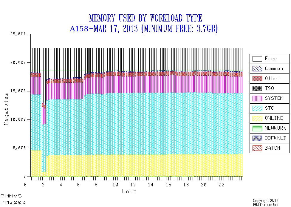
And PM2200 looked like this:

Notice how early in the morning the Online work got bounced. If this happens every day the nosey bit of me says “I’ve learned this customer likes to bounce their Onlines ever night”.

64-Bit Shared And Common

I hadn’t seen much usage of 64-Bit Shared or Common memory usage, despite DB2 V9 introducing a mandatory Shared 64-Bit memory object.

But then, and you probably guessed this one 🙂 , I got a set of customer data…

PM2200 – when first produced – looked simply awful[8]. The main problem with it is that not all the memory was accounted for. Further the supposed total memory was variable – which only really happens if you bring reserved memory[9] online and that’s a one-off event rather than continual variation.

A little guesswork suggested that maybe the discrepancy was 64-Bit Shared memory and 64-Bit Common memory. This turns out to be correct – and is corroborated by these two quantities appearing in the RMF Paging Activity Report.

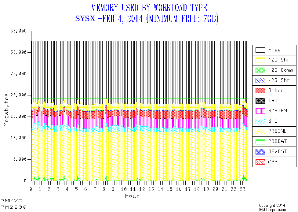
So I adjusted PM2200 to also show 64-Bit Shared and 64-Bit Common. In this case the Shared memory was about 6GB. The Common was small. Adding them in led to a constant total memory as well as that total being the same as the memory online to the LPAR – both of which are goodness.

The latest version looks like this:

Now this is a much less extreme case than the one that made me go “sacre bleu!”

You can extend the analysis for 64 Bit right down to the address space level: SMF 30 has numbers for 64-Bit Private the address space owns and the Shared Memory the address space can see.[10].

You can also work at the WLM Service Class level: SMF 72–3 has the Shared figure in it. I didn’t have SMF 30 for the 6GB case so I used SMF 72–3 to identify one Service Class (“STC”) as owning the shared memory. I also didn’t have useful report classes to work with so couldn’t narrow it down further. What I do know is this probably isn’t DB2 as there are other service classes with “DB2” in their name. But I can’t be certain about this without the 30’s.

In principle I could break down the Shared and Common numbers further – by workload – but I think you’ll agree the chart is already very busy. I have some more design work to do but I think it calls for 1 or more further charts.

---

You can probably see why I led with “do try and keep up”. This post outlines how one’s reporting has to evolve for two reasons:

• To wring all the insight you can out of the data.
• To adapt your reporting to technological changes.

But it’s a continuous struggle and I recognise most people don’t have the time to maintain their reporting too much. Arguably it’s my job.

---

And just as I thought I was ready to publish this post another piece of information comes up. I had a discussion with the MQ on z/OS Development lead Peter Siddall [11] about whether MQ uses Shared or Common 64-Bit objects. If you’re migrating to MQ 7.1 (perhaps from 7.0.1) you might want to pay attention to this:

MQ 7.1 requires the ability to create 64-Bit Shared memory objects: If you don’t allow that then MQ won’t start. The actual memory usage is generally small and MQ Development recommend a MEMLIMIT of at least 2GB. In any case the usage can be tracked by SMF 30 and so on.

(Originally posted 2014-02-23.)

As you might know I like maths, particularly algebra. (If you’ve read Another Neat Piece Of Algebra – Series Summation and Hello, I’m Martin And I’m An Algebraic 🙂 you do.)

If there’s one thing I would be doing if I weren’t doing this[1] it might be teaching maths – but it would have to be at a level where algebra and calculus were substantial topics. But I don’t think I’ll really be doing that – at least not for the foreseeable future. [2]

So it occurred to me that I need not be alone in treating some algebraic techniques as puzzles[3] – and with automatic generation of problems people could really get quite good at it. That might be useful – though utility is not my prime motivator in liking algebra: I almost never get to use it.

I won’t claim I was looking for a programming project: The day job gives me enough of those and anyway I have other ideas for fun stuff to create.[4] But anyway, this weekend I created a basic polynomial factorisation page. It’s a single file, containing javascript, HTML and CSS – which makes it quite portable.

After a brief preamble about factorisation and some hints it presents you with a machine-generated second-order[5] polynomial in x to factorise. You type in the factors and press the “Check” button.

The code multiplies the factors together and tells you what the resulting polynomial is. It also compares it to the original and tells you if you’ve got it right.

There’s a “Try another” button or you can just manually reload the page.

Try the code in here. You’ll have to paste it into your own HTML file and pop it in your browser.

It’s a little rough and ready. In particular you have to be little careful in how you type the factors in.

I’ve thought of some ways I could improve it already:

• I can think of difficulty levels.
• I could extend it to third- or fourth-order polynomials.
• I could extend it to polynomials in x and y.
• I could give tutorial hints.
• I could graph the resulting polynomial – probably on an HTML5 canvas.
• I could work on the text some more.
• I could use the HTML5 Offline Web Applications function to enable you to download it and run it on, let’s say, your smartphone.

But for now I’m enjoying testing it. And I hope you enjoy playing with it too.

And, in case you’re wondering, I have a memory-related “day job” post beginning to take shape in my brain.

.variable { font-style:italic; font-size: 125%; } .exponent { font-size: 75%; vertical-align: super; } .equation { background: #ccffcc; padding: 10px; box-shadow: 10px 10px 5px #888888; display: inline-block; } .bracket:before { content:”(“; } .bracket:after { content:”)”; } .wrong { color: #ff0000; } .right { color: #00ff00; } // Create HTML to display polynomial // Assumes: 1) All coefficients in array // 2) Lowest power of x first i.e. zero // 3) No leading-zero coefficients function showPolynomial(c,anchorID){ poly=’‘ for(i=c.length-1;i>=0;i–){ // Suppress 1 multiplier and last coefficient=0 cases if((c[i]==1) && (i>0)){ // Not c[0] and is 1 multiplier coeff=”” }else{ if((c[i]==0) && (i==0)){ // c[0] and 0 is multiplier coeff=”” }else{ // Normal case coeff=c[i] } } // Print term if non-zero coefficient if(c[i]!=”0″){ switch(i){ case 0: term=’‘+coeff+’‘ break case 1: term=’‘+coeff+’x‘ break default: term=’‘+coeff+’x‘+i+’‘ } // Figure out if we want a + before term if((c[i]<0)||(i==c.length-1)){ plusTerm="" }else{ plusTerm='+‘ } poly+=plusTerm+term } } poly=poly+’‘ anchor=document.getElementById(anchorID) anchor.innerHTML=poly } function multiplyPoly(p1,p2){ order=(p1.length-1)+(p2.length-1) var result=Array() for(p=0;p<=order;p++) { result[p]=0 } for(i1=0;i1<p1.length;i1++){ for(i2=0;i2<p2.length;i2++){ result[i1+i2]+=p1[i1]*p2[i2] } } return result } function polysEqual(p1,p2){ // Polynomials need to be of the same order if(p1.length!=p2.length) return false for(i=0;i-1){ poly[0]=parseInt(factorString.substring(plusPos+1)) return poly } // check for mx-n case minusPos=factorString.indexOf(“-“) if(minusPos>-1){ poly[0]=-parseInt(factorString.substring(minusPos+1)) return poly } // check for mx case if (factorString.substring(xpos+2)==””){ poly[0]=0 return poly } // Broken case return null } function checkIt(){ // Check first factor user might’ve typed in f1=parseFactor(“f1”) if(f1==null){ alert(“Type in the first factor – such as 2x+1 or 3x or x-1.”) } // Check second factor user might’ve typed in f2=parseFactor(“f2”) if(f2==null){ alert(“Type in the second factor – such as 2x+1 or 3x or x-1.”) } // If both factors are non-null proceed if((f1!=null) && (f2!=null)){ guessMultiplied=multiplyPoly(f1,f2) showPolynomial(guessMultiplied,”product”) yesno=document.getElementById(“yesno”) if(polysEqual(p12,guessMultiplied)){ yesno.innerHTML=”correct!” yesno.setAttribute(“class”,”right”) }else{ yesno.innerHTML=”wrong.” yesno.setAttribute(“class”,”wrong”) } document.getElementById(“prodDiv”).style.display=”block” } } Factorising Polynomials

Factorising Polynomials

Factorising polynomials is a basic but satisfying exercise in algebra. Try it here, with some random machine-generated examples.

Factorising is the process of turning a polynomial such as:

x2+3x+2

Into simpler factors. In this case they would be x+1 and x+2. If you multiply the two factors together you get the original polynomial.

Notice how the 3 in the polynomial is the sum of the 1 and the 2 in the pair of factors. Also how the 2 in the polynomial is the product of the 1 and the 2 in the two factors.

This actually wouldn’t be the case if the coefficient of the x2 term weren’t 1. But it’s not difficult to extend the thinking to cope with these cases.

---

And now it’s your turn.

Factorise:

3x2+8x+4

Write the two factors in the form 2x+1 or x or x-3.

Factor 1: Factor 2:

Check

Try another

(Originally posted 2014-02-19.)

In zIIP Address Space Instrumentation I discussed the subject of zIIP Capacity Planning.

What I was working on – but wasn’t ready to reveal – was a presentation on zIIP Capacity Planning. But I was also working on my new “zIIP CPU From Type 30” code. And that’s indeed what that post is about.

Now I am in a position to reveal my new presentation. You can get it from here. Usually I present a new set of slides at some conference or other, and then publish on Slideshare. This time I’m doing it the other way round.

Thst does, of course, present a small risk: It’s possible conference organisers will decide they don’t need me to present. I’ll take that risk as:

• I consider this material to be important to get out there.
• This is a living presentation.
• I think people want to hear me anyway. 🙂

The “important” bit is, ahem, important. 🙂 It relates to the fact that DB2 Version 10 changes the rules a bit: As I said in zIIP Address Space Instrumentation it’s the first zIIP exploiter that has especially stringent[1] requirements for access to CPU. This means you need to examine zIIP CPU more critically than ever. This message bears repeating, controversial as it probably is.

The “living presentation” bit relates to the fact that each customer situation teaches me something It’s a fair bet future ones will influence this presentation, without negating its essential thrust. Indeed several situations over the past three months have led to this presentation being better. I also have John Campbell and Kathy Walsh to thank for this being a significantly better presentation now.

Anyhow, feel free to read the slides and tell me what you think. And hopefully I’ll get to present the material a fair few times.[2].

(Originally posted 2014-01-15.)

Basic tutorial or advanced nicety? You decide…

Having been told what I thought was a nice high level presentation was “a bit too technical” I’ll confess to a perpetual (slight) anxiety about “level”. 🙂

Anyhow, this post is about inferences from LPAR names, particularly deactivated ones.

(If you catch me saying “inactive LPARs” I apologise. I mean ones that are defined on a machine but not activated, as opposed to those that are just idle.)

You probably know that RMF’s Partition Data Report lists activated LPARs by processor pool. (In some cases this can mean an LPAR appearing twice or thrice – if zIIPs or zAAPs are configured to the LPAR.) What you might not know (or might have ignored) is that the same report contains a list of deactivated LPARs.

As someone who majors on SMF data rather than RMF Reports (though I’m thoroughly conversant with the Partition Data Report) I’ve not reported on deactivated LPARs before. In our reporting we only list ones with some engines and memory defined.

A number of things have led me to believe understanding the defined-but-deactivated LPARs is handy:

• I see gaps in LPAR numbers I’d quite like to explain.
• I hear customers talk of recovering LPARs from one machine to another.
• I’d like to understand how much memory is hypothecated for currently deactivated LPARs.
• I’d like to understand whether an LPAR might be set up but be going to be activated later.

You could call these “nosiness matters” but I think they help tell the story.

What Do We Have?

In SMF 70 Subtype 1 (CPU Activity) we have two sections that are relevant to PR/SM and LPARs:

• PR/SM Partition Data Section
• PR/SM Logical Processor Data Section

The former has one for every LPAR defined on the machine, regardless of whether it’s activated or not. The latter has one for every logical processor, whether online (even if parked) or not. Deactivated LPARs have no logical processors, so no Logical Processor Data sections.

Up until now my code has merged Partition Data sections with Logical Processor Data sections and thrown away data for deactivated LPARs. Not any more.

But what you get in the Partition Data section for a deactivated LPAR is only a small subset of what you get for an activated one: You get the name and the LPAR number. That’s it (and I’m not complaining). You don’t get, for example, memory allocated – as there is none.

So I routinely report on the deactivated LPARs for each machine you send me data for. The table has their names and and numbers.

Nosiness Matters

(I have a presentation called “Memory Matters”. Perhaps I should have one called “Nosiness Matters”. 🙂 )

Back to my list of things I wanted to know about deactivated LPARs:

Missing LPAR Numbers

Unless you can tell me differently I see filling in the gaps in LPAR numbers a matter of tidiness. In any case the deactivated LPARs’ LPAR numbers let me do that.

Recovering LPARs

When I’ve used ERBSCAN and ERBSHOW to look at SMF 70-1 records (which I do as a diagnostic aid sometimes, and when developing new code) I see eerily familiar LPAR names.

For example, I might see CEC1 with an activated MVSA LPAR and CEC2 with a deactivated MVSA LPAR. It’s a reasonable guess that either

• The LPAR got moved permanently from CEC2 to CEC1 (and the definition was left unchanged).

or

• The intent is to recover MVSA from CEC1 to CEC2 if necessary.

I’ll admit I don’t know nearly enough about recovery strategies (outside of what Parallel Sysplex and some of its exploiters can do). But this should be a good conversation starter.

Hypothecated Memory For Deactivated LPARs

You don’t get, as I mentioned, memory for deactivated LPARs. This is because they don’t have any: It would be in unallocated memory (a figure RMF also doesn’t have.)

So my approach is to note the deactivated LPARs and enquire how much memory is notionally reserved for them. I can get the purchased memory from the machine’s Vital Product Data (VPD) and do the sums.

LPARs Not (Yet) Present

For some machines I see “aspirational” LPARs – such as ones with “LINUX” or “VM” in their names. Those would be ones the installation hopes to use at some stage. (I’d rather believe that than that the LPAR was the result of an unconvincing experiment.) 🙂

In one set of data I see two pairs of LPARs, one for each of a pair of demerging organisations. Each pair is Prod and Dev. Of these one “DEV” LPAR is deactivated. I guess Development has already moved off, leaving just the counterpart Production LPAR. (The other pair of Prod and Dev remain activated.)

Conclusion

You’ll spot not all my potential lines of enquiry are exhausted. But you”ll see I can make good progress – and ask a whole series of new questions. Hopefully you’ll see value, too.

I’ve also not talked about the panoply of different activated LPAR names. For example, having MVS1, IPO1, SYSA and C158 in the same machine says something about heritage. 🙂

(Originally posted 2013-12-13.)

Increasingly people are going to want to understand their zIIP usage and do capacity planning for zIIPs. Previously I’ve written about zIIP CPU numbers from the RMF perspective, namely at the WLM Workload and Service Class levels. This post is about taking it down a layer – to the address space level – using SMF Type 30 records.

(I’ve always thought it a pity there isn’t a standard reporting program for SMF 30, analogous to the RMF Postprocessor. But I digress.)

As you’ve probably gathered SMF 30 is one of my favourite record types. This post describes a few more ways you can get value from it. And some of those ways are, as you’d expect from me, more about nosiness about what customers are doing than about performance or capacity.

What We Have

First, a brief review of the zIIP-related numbers. (And just about everything I say in this post relates to zAAP as well.)

• For a very long time we had TCB and (Non-Preemptible) SRB time.

• A long time ago – when they were introduced – we had Preemptible SRB times – for Dependent and Independent Enclaves.

• When zIIPs were introduced we had zIIP-eligible and zIIP-eligible-but-on-a-GCP sets of times.

  The latter is the case where work was eligible to run on a zIIP but instead ran on a General Purpose processor (or GCP for short).

Both sets of zIIP times incorporate two buckets of time: for Dependent Enclaves and Independent Enclaves. I subtract these two numbers from the headline zIIP time. For example,

Other_zIIP = Overall_zIIP
           - Dependent_Enclave_zIIP
           - Independent_Enclave_zIIP

This is a useful thing to do – as we shall see.

zAAP On zIIP

zAAP On zIIP allows you to treat zAAP-eligible work as if it were zIIP-eligible. The benefit of this is that it gives you additional ways to fill up a zIIP.

From an instrumentation point of view, with zAAP On zIIP all the zAAP-related numbers become 0.

Address Space Characterisation

(My standard claim applies here: It helps a lot if you can get information from widely-available instrumentation without either asking someone or going to more specific data. In this instance it’s provided by SMF 30.)

Suppose you have an address space in mind – and it could be any Full Function address space:

• It could be a batch job, cutting SMF 30 Subtypes 4 and 5 when steps and the job end.
• It could be a long-running address space, cutting SMF 30 Subtypes 2 and 3 on an interval basis.
• It could be a terminating address space, in which all four subtypes should get cut at the appropriate points.

The point is it doesn’t matter which of the above applies. The fields I just described are always present.

Let’s pick on one example: The job name is immaterial but the program name is CTGBATCH (and zAAP on zIIP is in play). You might know this program name denotes the address space is running CICS Transaction Gateway (CTG). You might not know that much of CTG’s work is executing Java. (Non-JNI) Java work is zAAP-eligible but in a zIIP-but-not-zAAP environment it becomes zIIP-eligible. But it’s not work that runs in either a Dependent Enclave or an Independent Enclave: Its CPU falls into the “Other zIIP” category I just calculated. This would also be true of System XML processing (which is not Java).

Another example is DDF. The DIST address space is obvious to spot: Its job name ends in “DIST”, just as the corresponding DBM1 address space’s job name ends in “DBM1” (and the subsystem name is whatever precedes these two in the job name) . When some DDF work enters the system it is assigned to an Independent Enclave – but not until work such as authorisation has already taken place under TCBs. You can see the TCB time, the Independent Enclave time and the zIIP-eligible Independent Enclave time in SMF 30. The “Authorisation etc” time is the TCB time minus the Independent Enclave time.

Commonly we talk of the eligible percentage for DDF. That is the zIIP-eligible Independent Enclave time divided by the Independent Enclave time, converted to a percentage.

If you want to go deeper on this you do, of course, need to work with DB Accounting Trace (SMF 101).

An Important Case – DB2 Version 10

In DB2 Version 10 some performance-critical categories of work – Deferred Write Engines and Prefetch Engines – became zIIP-eligible. Note the words “ performance-critical categories of work”. This is the first time that phrase could be used with reference to zIIP-eligibility. And it’s right: If these engines don’t run in a timely fashion bad things happen.

The implication of this is we can’t fill zIIPs to the brim with this kind of work, and especially not if the LPAR has only one or two zIIPs.

If we do then either the work will get delayed because it can’t cross over to the General-Purpose Processors (GCPs) – and that will be a problem – or else it does cross over and we might get an unacceptable loss of zIIP benefit.

DB2 Lab recommends that, averaged over the peak 15 minutes (happily usually an RMF interval), you don’t run DBM1 zIIP utilisation for this work above 30 to 50% busy. The 30% number is for a single zIIP and the 50% number is for numerous zIIPs.

But what about “multitenant” zIIP usage? For example DBM1 plus Java work?

You can infill with less performance-critical work such as Java so long as you:

1. Classify DBM1 properly so WLM and SRM can protect it.
2. Classify this infill work appropriately.
3. Don’t load the zIIPs as heavily as you would GCPs.

So how do you identify this performance-critical DBM1 work? It’s actually not difficult as the work shows up in the Dependent Enclave zIIP Eligible CPU time. (And the amount that crosses over to GCPs is in an analogous time bucket – so yiu can check if this amount is acceptable or not.)

I’ve just mentioned how to tell if there’s too much crossover to GCPs. But what about the other problem area – work getting delayed? There are two places to look:

• In Accounting Trace for work being delayed. I’d expect it to show somewhere like the Read Asynchronous Wait and Write Asynchronous Wait buckets.
• In Statistics Trace with failures to get Prefetch and Deferred Write engines.

Note: Prior to PM30468 DB2 Version 10 scheduled these engines in a way that caused the CPU to show up under MSTR rather than DBM1. With the fix it’s in DBM1. (I’ve not seen it in MSTR.)

---

I hope you’ve seen how the various zIIP-related fields in SMF 30 can be used to understand the proclivities of an address space. More importantly, I hope you’re more aware than ever of the importance of zIIP capacity planning. And especially the added emphasis the new zIIP exploitation by DB2 Version 10, now it’s become a widespread version.

(I’ve had this post “in the can” for a couple of weeks and been sensitised in the meantime to some new things. All of which will appear in the “zIIP Capacity Planning” presentation I also have in the works.)

(Originally posted 2013-11-08.)

Usually a residency ends on the last day. Well doesn’t everything? 🙂

But this one’s been a little unusual in that regard. Straight after the residency came a week in which two of us presented at the GSE UK Annual Conference on aspects of the residency:

• Dean Harrison presented on Scheduling and JCL aspects.
• I presented on Performance aspects.

And Karen Wilkins, the other resident, was working the DB2 stream.

So, we got a chance to test reactions to some aspects of the book. We also collected a couple more reviewers.

I won’t mention any names here but my session in particular “lit up” when it came time to questions. And these got me thinking (which is why I love getting questions).

• There was a question about I/O bandwidth and increased parallelism. Yes, I think that has to be analysed and managed. And I should probably write something in the book about it. In our tests we didn’t actually manage to drive I/O in a way that caused time to be spent in the DB2 I/O-related Accounting Trace buckets. But I don’t feel bad about that as it’s impossible to construct an example that exemplfies everything and the technological lessons are fairly straightforward to grasp. (For reference they are in the area of I/O reduction and dealing with the remaining I/O hot spots in the usual ways.)

• There was a question about examining the whole environment into which you thrust this cloned workload. Again I should probably write something in the book about it.. And in our case it mattered because, not to spoil the story, the 32-up cloning cases led to CPU Queuing which limited our ability to scale effectively.

These two are actually questions I’ve addressed in previous Batch Performance Redbooks. So I don’t want to repeat myself very much. But they are important for cloning.

There was a third question which is worth addressing:

• Is there really anything new in this? The answer is: Not really, but people are increasingly going to have to pay attention to it, plus we have some nice techniques in the book (and Dean explained some of those in his presentation). We did the book because one is needed.

There was a fourth question or rather theme. We rather dodged it in the book. It’s really about how to treat whole strings of jobs. And I should probably write something in the book about it.

But it’s mainly about when to (and how to) “Fan Out” and “Fan In”.

When To Fan Out And When To Fan In

In the book we simplify things by writing about a single original job step that needs cloning. While that’s the right thing to do there are important considerations at the “stream of jobs level”.

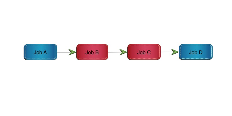
Consider the following simple set of 4 jobs:

Job A and Job D won’t be cloned for now. Job B and Job C will.

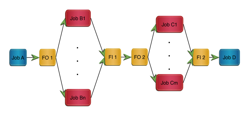
Here’s a naive implementation of what we recommend in the book: In this implementation Job B is replaced by FO 1, m clones and FI 1. Job C is replaced by FO 2, n clones and FI 2.

I don’t doubt we need FO 1 to fan out and FI 2 to fan in again, though both of these might be null. But do we really need to fan in after the Job B clones, only to fan out again before the Job C clones? There are a few reasons why we might not:

• From a scheduling point of view we wait for all the Job B clones to complete before we can start any of the Job C clones.
• Bringing data back together might be expensive.
• There are lots of moving parts here.

And that’s with just two jobs being cloned in the stream.

How Many Clones?

You’ll notice there are n clones of Job B and m clones of Job C. It’s probably best to standardise on one or the other for the stream. That might be a difficult judgement to make, based on each job’s cloning “sweet spot”. And it might turn out that actually n=2m is better than n=m, for example.

Data Sets Flying Everywhere

Another difficult judgement to make is how to handle inter-job data. This gets complicated very fast and has to be taken on a case by case basis – so I won’t inflict more diagrams on you. 🙂

As a relatively simply example we might need to write consolidated data in FO 1 to data set DSA (for some external purpose). I don’t see that as being avoidable but that needn’t stop the Job C clones. With care (and maybe technology) FI 1 might run alongside the Job C clones:

If Job C read data set DSA that Job B wrote then Job C1 might need to read data set DSA1 that Job B1 wrote, in parallel with FI 1 reading it. (Job FI 1 has to recreate data set DSA, in this scenario.)

Likewise Job Cn needs to read DSAn that Job Bn wrote, in parallel with FI 1 reading it.

The most obvious difficulty here is contention between the Fan In job (FI 1) and the readers (C1 … Cn). Whether this is serious or not depends on things like the quantity of data written.

One Obvious Scenario

One scenario I can see the “when to fan in and out” question coming up in is during the actual implementation: Job A might be cloned but the follow-on Job B not yet and its follow-on Job C not yet. It’s probably best to clone Job A then Job B then Job C (or all three at the same time). Cloning Job A and Job C but not yet Job B is not so good. So extend the sequence of cloned jobs outwards rather than doing it spottily.

---

See, I used the word “simplify” a while back: This stuff gets complicated very fast. And I don’t know how much complexity is worth delving into. The previous section is a first go at handling it. Any deeper and I don’t think we help the reader. (That’s you.) 🙂

---

I bolded the words “I should probably write something in the book about it” when I wrote them because it’s a key message from the GSE Conference: We have more work to do. I turns out I have the latitude to do just that, with the writing tools on my laptop, and perhaps a little time (some of it likely to be on aeroplanes).

The conventional wisdom is that when the residents go home no more writing can be done. That’s probably a fair assumption but in this case I think it’s a little pessimistic. Or at least I hope so.

I’m tremendously proud of what Dean, Karen and I have achieved over our four weeks in Poughkeepsie. If you read the book, even in the state it’s in now, I think you’ll like it.

Technically we probably could go on for ever, adding stuff to it. One day that’ll have to stop – as we really do want to get the book out soon. (And actually I’d rather like to work with some customer applications in the vein of what we’ve written – but I don’t control my workload enough to insist that happens soon.) But for now the writing goes on.

Now where can I shove some more “Galileos”? 🙂

(Originally posted 2013-10-20.)

While writing Creating JSON with DFSORT I realised one statement in particular is difficult to read and maintain. It’s this one:

    INREC IFTHEN=(WHEN=INIT,BUILD=(SEQNUM,4,BI, 
              C'{"name": "',NAME,C'","number": "',NUMBER,C'"}')),
            IFTHEN=(WHEN=(1,4,BI,GT,+1),BUILD=(2X,C',',5,70)), 
            IFTHEN=(WHEN=(1,4,BI,EQ,+1),BUILD=(2X,5,70)) 

It’s not the first one that’s become complicated: Increasingly people are realising the power of what you can do with DFSORT – especially if you use multiple stages with IFTHEN. So complexity can become a real issue.

This post is the result of some thinking about how to make developing, reading and maintaining DFSORT applications a little easier. (And everything I say here is applicable to ICETOOL as well.) In a nutshell:

• Map the input records with symbols.
• Use symbols for intermediate fields.
• Consider symbols for combined fields.
• Use indentation.
• Build applications from the front to the back in stages.
• Consider using “dummy” IFTHEN stages.
• Use OUTFIL SAVE to avoid losing records.

The rest of this post expands on these.

Map The Input Records With Symbols

Whether you use COBDFSYM (in Smart DFSORT Tricks) to map COBOL copybooks or code your own by hand you should map the input records using DFSORT symbols. This makes the DFSORT invocation much more readable and a little more maintainable.

That’s actually what I did for the example in Creating JSON with DFSORT and if it’s readable that would largely be why.

(On COBDFSYM I wrote about it further in “Chapter 23.4.1 Converting COBOL copybooks to DFSORT symbols” of SG24–7779 Batch Modernization on z/OS.)

Use Symbols For Intermediate Fields

If you have, say, two fields NAME and NUMBER in your input record and you move them around or reformat them or otherwise mess with them consider remapping the modified record. Code

POSITION,1

to reset the Symbols pointer and then start mapping the modified record. Here’s something I tend to do:

If the original field is called NAME I create a new field in the remapping called _NAME. Similarly NUMBER becomes _NUMBER.

If I modify them again they become __NAME and __NUMBER. And so on.

(By the way the underscore characters in the above are written in Markdown by prefixing them with a backslash. I learnt that the hard way.)

Consider Symbols For Combined Fields.

If you are manipulating sets of fields consider using a symbol to describe them as a group. For example you might have formatted an intermediate form of the record with NAME followed by a blank followed by NUMBER. The Symbols deck might look like:

_NAME,*,8,CH
SKIP,1
_NUMBER,*,8,CH

But you could code an additional symbol:

_NAME_AND_NUM,*,17,CH
_NAME,=,8,CH
SKIP,1
_NUMBER,*,8,CH

And then you can use it as a combined field. The trick here is to use = to specify remapping. It positions the Symbols cursor back to the start of the first field.

In general * and = are very handy in Symbols decks. In brief

• * in the position field means the symbol’s position is just after the end of the previous symbol.
• = in the position field means it’s at the beginning.
• = in the length field means use the same length as the previous symbol’s.
• = in the type field means use the same type as the previous symbol’s.

Use these wherever you can and it should help maintainability.

Use Indentation

Instead of coding

     ...
  IFTHEN=(WHEN=INIT,BUILD=( ... )),
  IFTHEN=(WHEN=(...),FINDREP=(...)),
     ...

try coding something like

     ...
  IFTHEN=(WHEN=INIT,
    BUILD=(...)),
  IFTHEN=(WHEN=(...),
    FINDREP=(...)),
     ...

and it’ll be a little clearer.

You might also want to do something like

   INREC FIELDS=(NAME,
     RANK,
     NUMBER,EDIT=(IIT),
     ...

indenting the fields where possible and putting each on its own line. (You could indent the EDIT in the above but I think that’s going too far.)

Build Applications From The Front To The Back In Stages

Sometimes – and the past few days have been a good example of this – it takes a long time to debug a DFSORT application. The main reason is not understanding how the various stages – whether INCLUDE, OMIT, INREC, SORT, SUM, COPY, MERGE, or OUTFIL fit together. (And I’ve probably missed one or two out.) It’s even more complex with IFTHEN.

So I recommend building up the set of instructions, and within them IFTHEN stages, slowly. Check the output at each point is what you expect – before you build the next stage (which relies on it).

It sounds obvious but I labour the point as this stuff is getting complex and it’s easy to make mistakes. (Most of these are fuzzy understandings of what DFSORT will do.)

Consider Using “Dummy” IFTHEN Stages

This is a minor point and might be slightly controversial. Don’t do it in Production if you’re squeezing every last ounce of performance out of the application – but I seriously doubt it’ll be a problem.

Consider the statement:

INREC
  IFTHEN=(WHEN=INIT,
    BUILD=(...))

The bad news is it’s not legal DFSORT syntax and you’ll get a syntax error. The following, however, is legal:

INREC IFTHEN=(WHEN=INIT,OVERLAY=(5:5,1)),
  IFTHEN=(WHEN=INIT,
    BUILD=(...))

The first WHEN=INIT actually doesn’t change any records. Well it does but in a null fashion:

It replaces the byte at position 5 with the contents of the byte at position 5. 🙂 The net effect is to leave the record unchanged. If you can’t stand the first effective IFTHEN not being indented then this gets round it. More seriously you can move the effective IFTHENs around without having to mess with indentation.

As I said this is unlikely to affect performance. But if you think this trick obscure don’t use it. I just think it helps with maintaining indentation.

Use OUTFIL SAVE To Avoid Losing Records

If you are routing different records to different OUTFIL destinations – using OUTFIL’s own INCLUDE or OMIT parameters – it can get complicated to ensure all the records go somewhere. OUTFIL SAVE routes the records that don’t meet any previous OUTFIL INCLUDE/OMIT criteria to another DD. This saves coding complex “everything else” rules – even if Augustus De Morgan did found your Maths Department and you do understand Relation Algebra. 🙂

Note: The records thrown away by INCLUDE or OMIT statements can’t be recovered using OUTFIL SAVE.

---

As I say, writing the previous post reminded me of how ungainly the coding can be. But I didn’t think a list of techniques to handle that belonged in the same post. Hence this one.

If you have other DFSORT comprehension and maintainability tricks I’d love to see them. If you think these aren’t right – especially the last – let me know.

(Originally posted 2013-10-18.)

This post is yet another spin off from the residency I’m on in Poughkeepsie.

I mentioned in We Have Residents! I might do something with JSON (Javascript Object Notation) and indeed I have.

But why would a residency on Batch Performance concern itself with JSON (and indeed XML, which I’ve also written about in the Redbook)?

The reason lies in the word “modernisation”. This actually works two ways:

• Effective job cloning – where there is some kind of “printed” output – requires breaking the report data generation and report formatting into separate pieces. This is because there’s a need to fan in the reporting data. This re-engineered data flow provides the opportunity to publish the data to new consumers. If we’re going to do that it might as well be something nice and modern like JSON or XML. I’ve talked about XML before – so I won’t in this post.
• Modernising batch jobs means opening the code up anyway (and that might indeed be to produce new formats of output) so it would be good to consider whether it should be parallelised. And the most obvious way is by cloning it.

Now obviously not all batch jobs want modernising or cloning. But some in an installation probably do.

---

So below is a simple example of using DFSORT to create JSON from SYSIN. Consider the following JCL:

    //MAKEJSON EXEC PGM=ICEMAN 
    //SYSOUT   DD SYSOUT=* 
    //SYSPRINT DD SYSOUT=* 
    //SYMNOUT  DD SYSOUT=* 
    //SYMNAMES DD * 
    POSITION,1 
    NAME,*,8,CH 
    SKIP,1 
    NUMBER,*,8,CH 
    /* 
    //SORTIN   DD * 
    ALPHA    ONE 
    BRAVO    TWO 
    CHARLIE  THREE 
    DELTA    FOUR 
    /* 
    //SORTOUT  DD SYSOUT=* 
    //SYSIN    DD * 
    OPTION COPY 
    * 
    INREC IFTHEN=(WHEN=INIT,BUILD=(SEQNUM,4,BI, 
              C'{"name": "',NAME,C'","number": "',NUMBER,C'"}')),
            IFTHEN=(WHEN=(1,4,BI,GT,+1),BUILD=(2X,C',',5,70)), 
            IFTHEN=(WHEN=(1,4,BI,EQ,+1),BUILD=(2X,5,70)) 
    * 
    OUTFIL FNAMES=SORTOUT,REMOVECC, 
     HEADER1=('{'/, 
    '"inventory": ['), 
    TRAILER1=(']',/, 
    '}') 
     END 
    /*

On my system it produces:

{
"inventory": [
  {"name": "ALPHA   ","number": "ONE     "}
  ,{"name": "BRAVO   ","number": "TWO     "}
  ,{"name": "CHARLIE ","number": "THREE   "}
  ,{"name": "DELTA   ","number": "FOUR    "}
]
}

If you put that through a JSON validator, such as JSONLint it is reported as clean JSON. (This particular service reformats it prettily as well.)

There’s a trick here, though, that’s worth describing:

JSON is picky in that – for elements or arrays – you have commas in between but you can’t have a leading or a trailing comma separator. (This actually isn’t always true of Javascript but was enforced for (the derivative) JSON.

All the interesting action is in the INREC (could’ve been OUTREC or even OUTFIL OUTREC) statement. This has three IFTHEN clauses (or stages if you prefer):

1. Always fires. Produces the formatted line with a 4-byte sequence number on the front. The sequence number starts at 1 and is in binary format.

2. Fires if the sequence number is greater than 1. Places a comma (and two indenting spaces) in front of the formatted line.

3. Fires if the sequence number is 1. Just places the two spaces (and no comma) in front of the formatted line.

I say “trick” but this is just the standard “treat each record according to its characteristics and through multiple stages” approach you can take with DFSORT IFTHEN.

In any case it produces 1 line without a comma and the following ones with a comma. And JSON rules are satisfied.

---

By the way you might be wondering why the values are capitalised or have trailing spaces. This is actually preserving what was in the original records (in in-stream SORTIN). You can certainly take trailing spaces out but it needs a little more work. Semantically both belong in the output data, of course.

And if you insist on taking trailing spaces off the lines – as opposed to out of the items – you can always use DFSORT’s VLTRIM.

I think it looks a little odd to have the separator commas at the beginning of the lines. But I don’t know of a way in DFSORT to test for the last line – to avoid placing a comma on it. If you can think of a way let us know.

But for now we have valid JSON that any JSON reader – whether raw Javascript, a framework like jQuery or Dojo, or some other language – can process.

And yes it would be nice to breathe new life into old data.

And – below the line 🙂 – is a brief discussion on JSON itself.

---

JSON is a spin-off from javascript. As I mentioned above you can process it with javascript by assignment. The following is entirely valid:

var inv={
"inventory": [
  {"name": "ALPHA   ","number": "ONE     "}
  ,{"name": "BRAVO   ","number": "TWO     "}
  ,{"name": "CHARLIE ","number": "THREE   "}
  ,{"name": "DELTA   ","number": "FOUR    "}
]
}
alert(inv.inventory.name[0])

which would – in a browser pop up a message box with “ALPHA” in it.

You mightn’t want to do that as you can end up executing arbitrary code. So direct assignment should only be used where you can trust the JSON. Which is why people tend to use libraries to parse it – and the good ones don’t do direct assignment.

People like JSON because it’s easy to generate, less verbose than XML, and now has a lot of ways of processing it. What’s not so good is that there is no notion of things like namespaces and schemas – so perhaps not so good for “Enterprise”. And it doesn’t have transformational tooling like XSLT. But it’s very popular.