(Originally posted 2014-05-03.)

Sometimes I’m in the mood to carefully peck at the text and sometimes I’m in the mood to just “splurge write”. And sometimes a bit of both.

This post is a case in point: I just want to get the words out as fast as I can.

Now, I do quite a bit of writing on iOS as it lets me write wherever and whenever I get the chance. I like its prediction and correction capabilities. But the app I want to talk about in this post takes that a good deal further.

It’s SwiftKey – available on iPhone and iPad alike.

You type and it presents three alternative words to choose from, as shown below.

Of course I chose the middle one.

It often predicts the words before you complete typing a word and sometimes you don’t even have to tap a word for it to be chosen.[1]

In my experience the accuracy of prediction is high, especially if you let it read your Evernote account to glean your writing style. It also learns from what you type in the app: So, in the example in the screenshot it has learnt that the word “choose” is often followed by “from”.[2]

I find whether I use a Bluetooth or an on-screen keyboard I can type much faster – which is a good thing as my brain often overruns my ability to type.

SwiftKey doesn’t understand (Multi)Markdown so it’s not much use for formatting. But recall one of the strengths of MultiMarkdown is the lack of formatting commands when writing paragraphs. Markup can often wait.

Unfortunately you can’t use SwiftKey as the standard text entry subsystem for apps in general. So I find myself cutting and pasting the text into other apps, such as Editorial. This is only a minor pain in fact: I’m still getting ideas down very fast. But it would be nice if Apple allowed customer data input mechanisms.

In fact you can use SwiftKey as a fast test entry mechanism for Evernote as it can save notes directly into Evernote. In fact I don’t do that: Most of my Evernote notes come from elsewhere (and have a good deal more structure.) Perhaps I’ll write about that one day.

So this is the fourth in a series about apps I use. The previous one was Appening 3 – Editorial on iOS. My reviews aren’t as comprehensive as many you’ll find on the web but they are more insights into how I use stuff than formal reviews. Of course this isn’t an official IBM endorsement of SwiftKey: I’m just telling you about a tool I use and what I think about it.

(Originally posted 2014-05-02.)

If you have a large mainframe estate it can be difficult to keep track of when the various moving parts start and stop. For example, if you’re a Performance person it’s quite likely nobody bothered to tell you when the systems were IPL’ed. You might well know what the regime for starting and stopping CICS is but I wouldn’t.

As you know I’m curious as to how customers run their installations and starting (and stopping) pieces of infrastructure interests me. I’m also impressed when a piece of infrastructure has been up for years – as sometimes happens. Up until now it’s been a matter of folklore such as “the installation that didn’t take an application down for 10 years”.[1]

But I’ve turned my attention to when z/OS is IPL’ed and when key address spaces start and stop. I’m sharing the technique in case it’s something you want to do.

I’m also interested in the sequence and timing between a z/OS system’s IPL and when important subsystems are up.[2]

I’m not going to pretend to be an expert in how systems are restarted or recovered but I am going to take an interest. Knowing what’s “normal” is, I think, useful.

Simple Instrumentation

You probably know that SMF 30 subtypes 4 and 5 describe steps and jobs, respectively. You probably also know SMF 30 subtypes 2 and 3 are interval records.

If you’re already collecting these you’re in good shape as Reader Start Time is in all of these. It’s all you need to figure out when stuff starts.[3]

I prefer the interval records as

• Most customers send me SMF 30 interval records. (I get the others for batch studies.)

• You can get the Reader Start Time from these even when the address space is still up. (When the Reader Start Time changes for an address space I know it’s restarted.)

Summarisation And Reporting[4]

For some address space types I report each job name separately. CICS regions are a good example of this. For others I pick the first one for a subsystem. DB2 and MQ subsystems are a good example of this.

To detect an IPL I choose the address space whose program is IEEMB860. In principle the job name could vary. And yes I know that “pressing the button” on IPL invokes NIP etc before this (the Master Scheduler) address space starts up.

I only print date, hour and minute for Reader Start Time. It goes to hundredths of seconds but I’m not interested in that level of detail.[5]

In my report I sequence by timestamp. That makes it easier to see when an IPL is followed by, say, a DB2 start and then some CICS regions. I could probably create a useful Gantt chart from this, but today I don’t. The technology’s there to make this easy to do.

Conclusion

Looking at this data gives me a much better idea how installations manage the lifecycles of their address spaces. If I talk to you about this topic it’ll probably be from this data and I might well refer you to this blog post. This is also one of the topics in the 2014 revision of my “Life And Times Of An Address Space” presentation.

Two final points:

• Reader Start Time doesn’t denote the time that a subsystem became available, so it’s not that good for application availability. You probably want to use the subsystem’s own instrumentation, such as logs, for that.[6]
• One of the merits of the Reader Start Time technique is that it’s very “light touch”.

(Originally posted 2014-05-01.)

Over a year ago I wrote about a couple of iOS applications I was enjoying using.[1]

And now it’s time to write about a third, as it’s part of my authoring toolkit. In Recent Conference Presentations I showed off my then new writing rig: Byword (with MultiMarkDown) and my iPad Mini with a Logitech light keyboard cover. I said that would be my rig for a while.

So this post also serves to talk about my current writing setup. The hardware has changed a fair amount: I still use the iPad Mini in lots of places but now I’m using my iPhone for writing in tight spots and a new iPad Air for where I can spread out a bit more.

The software has changed as well: I use Byword on the Mac for final editing and use it less on iOS devices. That’s because I have a new writing tool on the iPads: Editorial, which also does MultiMarkDown. The “secret sauce`” in Editorial is the ability to write what are called workflows. Some of these are drag and drop essentially pipeline stages. But, and this is where my interest really takes off, you can write workflows in Python.[2]

Those of you who follow me on Twitter might’ve spotted me talking about building workflows with Editorial. The two most notable ones – both built in Python are:

• A workflow to check footnotes are properly defined and actually get referenced. (It actually sorts the footnotes by first reference – which is useful for authoring but redundant when it comes to converting the MultiMarkDown to HTML.)

• A workflow to check I’ve created the images I reference – or at least that they exist on the iPad.

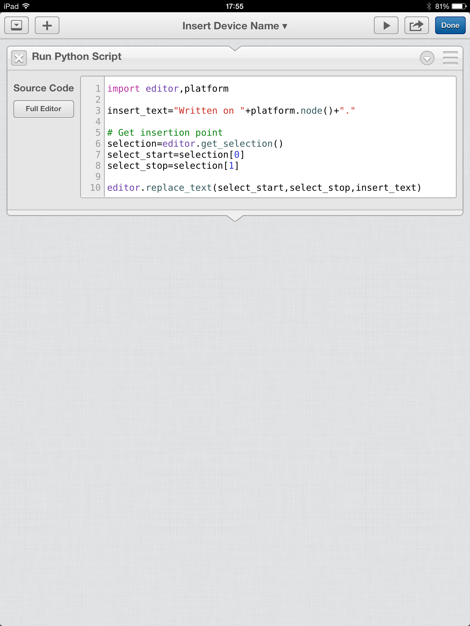
But here’s a simple workflow. It does a (probably useless) thing of inserting the name of the iOS device into your document’s text at the cursor. The workflow has only one “stage”, a Python script[3]:

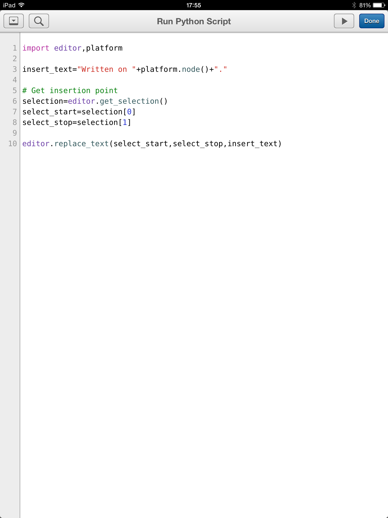
This looks like “keyhole surgery” but clicking on the full editor yields

and then you can edit, with some very nice syntax assistance and module prompting, to your heart’s content.

When you run this the words “Written on FunfPad[4].” are inserted into the text. Actually, if you have selected range of text it will all be overwritten with these words.

Of particular note here is the editor module – which gives tight integration between Python and the editor. Others such as workflow round the integration out nicely.

There’s a nice little community for discussing Editorial (including with the author) at omz:software Forums.[5] I’m learning a lot from this community.

I’m also using Dropbox to keep posts and graphics I’m working on. This enables me to work on them across Linux, OSX and multiple iOS devices. (I have no reason or appetite to write on Windows.)

So, you can see my writing toolset is evolving, and no doubt it will continue to. By the way this is my personal view and experience, rather than an IBM endorsement. But I’m sure you realised that.

(Originally posted 2014-04-30.)

I’ve been meaning to write about MEMLIMIT and its importance for some time.[1]

But it’s a moving target. So either there’s no good time to talk about it or lots of good times. 🙂 So let me discuss it now and then again later as necessary.[2]

So timing a post on MEMLIMIT is like choosing a wave to catch: In this case the wave was a discussion in IBM-MAIN about where to find out the MEMLIMIT for an address space, plus the way the MEMLIMIT value came to be set for that address space. Or maybe it’s the announcement of MQ Version 8, which does move the folklore on a bit.

So let me start by describing what MEMLIMIT is and why it’s important. Then I’ll talk about a few examples. Finally I’ll talk about instrumentation.

Why Is MEMLIMIT Important?

Nobody cares how much virtual storage you use, so long as you don’t cause real world effects.[3]

Real world effects include overuse of real memory – as it’s not free – and overcommiting real memory and, still worse, paging space.

MEMLIMIT is the mechanism for limiting an address space’s use of virtual storage. It can be set on the JCL EXEC statement, via an IEFUSI installation exit or in SYS1.PARMLIB(SMFPRMxx).[4]

One way or another you have to set MEMLIMIT for each address space:

• Set it too low and the address space might refuse to start. Here I’m thinking of specific products.

• Set it too high (or to Unlimited) and you create an exposure: Someone could create a vast 64-Bit Memory Object and touch every page, potentially causing the system to die.[5]

A good but old document on MEMLIMIT is Limiting Storage usage above the bar in z/Architecture by Riaz Ahmad.

Some Key Products

Let’s talk about CICS, DB2 and MQ.

CICS

In a typical CICS environment there are numerous CICS address spaces. In CICS 4.2 the minimum value of MEMLIMIT is 4GB, else the CICS region won’t start. In CICS 5.1 the minimum is 6GB.

In reality CICS will use what it needs to. But a region might in fact need more virtual storage, so do keep track of its usage: SMF 30 can help.

DB2

There are generally few DB2 subsystems. The only really big address space is the DBM1 address space. Nowadays the MEMLIMIT is set in the JCL as 4 Terabytes. Don’t change it: DB2 can be trusted not to use a threatening amount of real memory, so long as you do due diligence on real memory.[6]

MQ[7]

Again there are relatively few MQ subsystems but usually the big address space is MSTR. In Version 7 the default MEMLIMIT was set at 2GB in the JCL.[8]

In Version 8 things can potentially change, and you might need to increase the MEMLIMIT value: While buffer pools are by default still 31 Bit you can choose to make them 64 Bit (and you can long-term page fix them). If you make them 64 Bit you will need to review MEMLIMIT:

I’d suggest adding the sizes of the 64 Bit buffer pools plus 10% [9] to 2GB and setting that as your new MEMLIMIT.

Actually the CHIN address space can be pretty big, particularly if you have a large number of external connections. But it remains 31 Bit.

Instrumentation

As you might expect , SMF 30 (all subtypes) has the eventual MEMLIMIT value (in MB) for the job step. It also has the method by which the MEMLIMIT value was established.

I report on both of these at the address space level. And looking at this data gives me a much better idea how installations manage MEMLIMIT in general. If I talk to you about your MEMLIMIT approach it’ll be from this data and I might well refer you to this blog post. And I’m certainly talking about this in the 2014 revision of “Life And Times Of An Address Space”.

 

(Originally posted 2014-04-26.)

I’ll admit I’ve found regular expressions a bit of a struggle. I bet most people have. For me it’s a matter of lots of arcane symbols that don’t have any inherent meaning. Contrast with many programming languages, which do have some.

It’s also not the case I don’t understand the concepts.

Anyhow I’m edging towards the point where Production code will need to allow regexes. So I want to take a list of space-separated names and see which items match a given regular expression.

For example a list of address space names.[1].

And so the FL (for “Filter List”) REXX EXEC was born.

The code is below. It uses grep to do the testing and BPXWUNIX invokes grep.

You invoke it with

TSO FL <regex> <list>

if you’ve put it in a suitable CLIST library. Mine is in my ISPF one. I can also call it from ISPF Option 6 or from Batch.[2]

For example

TSO FL CICS$ CICSA CICSB PRODCICS MYCICS

Will display the string

PRODCICS MYCICS

as these two items match the regular expression.

/* REXX */
parse arg mygrep mylist

/* Create a temporary stem set with data to pass to grep via BPXWUNIX */
wds=words(mylist)
do w=1 to words(mylist)
  tmpStem.w=word(mylist,w)
end 
tmpStem.0=wds

cmd='grep "'mygrep'"'

/* Do the actual grep */
call bpxwunix cmd,tmpStem.,filter.,stderr.

/* Turn returned stem set into space-separated list */
resultList=""
do f=1 to filter.0
  resultList=resultList filter.f
end

/* Print any error messages */
do e=1 to stderr.0
  say stderr.e
end

say strip(resultList)

exit

Obviously this could be modified to be a callable routine, or to use one. In this simple sample I thought it best to leave it as open code.

You could probably also find a way to pass parameters to grep like -i for case insensitivity.

One further refinement which is more of a stretch is handling list items with a space in them: You’d need to rewrite the bit that creates stem variables from the words in the list string. But for my purposes I’m looking at names which don’t have spaces in them.

Observant readers will spot this code is derived from Filtering REXX Query Results With BPXWUNIX but this version is easy to prototype with from the command line.

If you’re wanting to get started with regular expressions have a play with it. Enjoy!

(Originally posted 2014-04-14.)

This post adds some additional DB2 Version 10 specifics to what I mentioned in New zIIP Capacity Planning Presentation. I said this would be a living presentation, and so it has proven to be. It’s had two outings so far and there are a couple more confirmed.

First the times I’ve given it:

• On 9 April 2014 I was very pleased this was the very first presentation given at the GSE/UKCMG zCapacity Management and zPerformance Analysis Working Group in IBM South Bank.
• This past week I tried it out as the jumping off point for a single-company discussion on zIIPs.

Now what’s ahead:

• I’m using the material again in another single-company setting. I’m quite keen the material can be used this way as I think a lot of installations will want to think the subject through.
• At the System z Technical University, 12 – 16 May in Budapest, I’m presenting to a (hopefully) much larger audience. Do come along if you can!

So since after these two outings I’ve extended the presentation by a couple of slides – and it’s these new topics I want to discuss in this post. They are:

• Subcapacity General Purpose Engines (GCPs)

and

• DB2 DBM1 zIIP Eligibility levels in DB2 Version 10

Subcapacity General Purpose Engines

I’m seeing quite a few installations with “subcapacity general purpose engines” – such as zEC12 Model 6xx processors. As you probably know with these the effective capacity of the GCPs is less than that of a 7xx but the zIIP (and ICF and IFL) engine capacity is the same as that of a 7xx GCP engine.

For example a z196–6xx has GCPs that are roughly half the speed of the zIIPs. And a zEC12–5xx would be a little more than 1/3 the speed of the zIIPs[1].

Having a faster zIIP than GCP can be good news as each zIIP could process CPU-intensive work faster and has more capacity. On the other hand when zIIP-eligible work runs on a GCP (as it might do in times of zIIP Pool stress) stuff (maybe “CPU Stringent” stuff) will run slower – introducing variability.[2]

It’s tempting to configure fewer zIIPs than you might if they’re, say, three times faster than the GCPs. I’d be cautious about that – because of the queuing effects[3] and the drop in performance that running zIIP-eligible work on a GCP might bring.

DB2 Version 10 zIIP Eligibility

One discussion I had was about an imminent migration from DB2 Version 9 to Version 10. In this case the use of zIIP by DBM1 is entirely new. My off-the-cuff response was to estimate the whole of DBM1 going to zIIP upon migration. This is, as you would probably guess, an overestimate. But it’s good enough for checking you have enough zIIP capacity to take the additional demand.

But I went back to the data I have from two DB2 Version 10 customers:

• Client A has no zIIPs.
• Client B has zIIPs.

After a head scratching moment I was pleased that I had both cases: The data appears to behave differently in the two cases, but in reality it’s consistent.

Here’s the unifying piece of information – that got me beyond head scratching:

Field SMF30CPT – which contains TCB and similar – includes zIIP-eligible work that runs on a GCP. It doesn’t contain zIIP-eligible work that actually does run on a zIIP.

Client A

The following is a graphic I already had in the presentation. (You might want to pop it into a separate tab in your browser.)

As I said they have no zIIPs so all zIIP-eligible work is included in the TCB number in the table.

If you look at the “DSNRDBM1” row in the table you see the TCB is 1.0% of an engine and the zIIP-on-GCP number is 0.84% of an engine. All the Dependent Enclave CPU is zIIP-eligible[4].

So somewhere between 80 and 85% of all the DBM1 CPU is zIIP-eligible – dividing 0.84 by 1.0 or so.

By the way, SRB is tiny so I’ve not displayed it.

Client B

Remember Client B does have a zIIP.

Again, any zIIP-on-GCP CPU would appear in the TCB number – but here it’s tiny. All the zIIP-eligible work does indeed run on a zIIP, so isn’t included in the TCB value.

As a one-off [5] I’ve created the following graph that explores zIIP-eligibility by time of day. I’ve added it to the presentation.

It shows generally zIIP-eligibility is in the region of 70 – 80 % of the total, consistent with Client A. The reason for creating it was to see how much the zIIP-eligibility varies. For this customer there is some variation and indeed a few sekips[6]. These, if one were to take the trouble to explain them, would probably turn out to be periods of low Prefetch and low Deferred Write. One might hazard a Direct and Read-Only situation could lead to a much lower level of zIIP-eligibility.

So, I would think it reasonably important to measure what proportion of DBM1’s CPU is zIIP-eligible but expect it to be in the region of 3/4. If you’re going to Version 10 from Version 9 I would provision enough zIIP CPU to support 100% but expect rather less.

---

I’ve enhanced the presentation with the above and that’s what I intend to give in Budapest and use in this next customer discussion. It might evolve a bit in the meantime – and that’s OK. The next version going up on Slideshare will probably be after Budapest, so mid May.

And I already know I need to do some work on the changes on DB2 Version 11 which promise more DB2 zIIP eligibility: I haven’t done the research yet.

(Originally posted 2014-04-01.)

There’s been some interest recently in whether a zBC12 as a standalone Coupling Facility would be a good idea. Having replied to one such question in email form I can count that as a draft for a blog post on the subject. It’s a complex question as are most about Parallel Sysplex configuration design. So this won’t be a comprehensive answer but I hope it’ll give you food for thought and perhaps a new way of looking at the relevant performance data.

There are two main themes worth exploring:

• What a stand-alone zBC12 allows you to do
• Signalling sensitivity to technology options

The second of these is a particularly boundless discussion. So let’s get started: I have a kettle to boil that ocean in. 🙂

A Stand Alone Coupling Facility

Consider the case of a twin-ICF[1] Parallel Sysplex environment where all the members are on the same pair of physical machines as the two ICFs.[2]

There are two design choices:

1) Duplexing [3] key structures across the two ICFs,

2) Not duplexing the structures.

The first choice is, thankfully, far more common than the second. It enables far higher availability and much greater resilience.

Consider the oft-cited case of a 2-way DB2 Data Sharing[4] Group where the LOCK1 structure is unduplexed and on the same footprint as one of the members[5]. Suppose this footprint suffers a hardware failure: Both the LOCK1 and one of the members fails and you’re in for a painful wait while the entire Data Sharing group restarts.

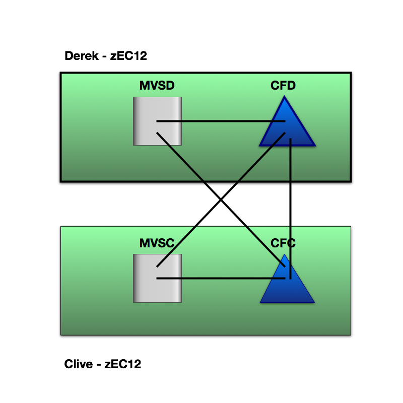
Here’s what a duplexing scheme looks like. It’s symmetrical. Often the two machines are in separate machine rooms some distance apart, but sometimes they’re sat next to each other.[6]

If instead you place the vital structures in a standalone zBC12 you would need both the zBC12 and one of the coupled machines to fail to cause the same group-wide restart.

Here’s what a standalone configuration could look like:

I’ve drawn the zBC12 (“Bairn”) nearer to “Derek” as in practice I don’t tend to see a third data center just to house the standalone CF. “Nearer” usually means shorter request response times, so we no longer have symmetry of outcomes between the two coupled members. This might matter.

There are, of course, other similar designs. One of these is a third footprint’s ICF where the other LPARs on that third footprint are in a totally separate parallel sysplex. To talk about these possibilities further would unnecessarily complicate an already long blog post.

One disadvantage of a stand-alone CF is that all the links between the coupled z/OS LPARs and the coupling facility are external, though this need not be an overwhelming disadvantage.

The rest of this post addresses how moving from a pair of ICFs affects performance.

Signalling Sensitivity

The key question is whether high-volume structures have good performance from the point of view of the coupled applications.[7]

When I examine a Parallel Sysplex environment I like to see data from all the members.[8]

To answer the question “would a slower-engined zBC12 suffice?” it’s necessary to understand what part CF engine speed plays in signalling and what the traffic is.

For a long time now RMF has reported Structure Execution Time (or, informally, structure CPU Time).[9] Assuming requests from one member to a structure take the same amount of CF processing as another we can estimate non-CPU time:[10]

If you subtract the CF CPU time for a request from the response time as seen by the member you get a reasonable view of the time used by queuing and signalling. You can’t really break these two out but they do between them represent the time not represented by the CF engine.

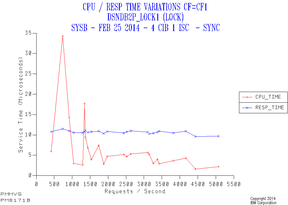
As an example consider the following case of a lock structure (DSNDB2P_LOCK1) in CF1 accessed by a member (SYSB) over a mixture of 4 Infiniband links and 1 ISC link[11]. All the requests are synchronous.

Along the horizontal axis is the request rate from the member to the structure. The red line is the CF CPU time per request, the blue being the response time.

• While the CPU time per request appears high at low traffic this is really an amortisation effect as there is a certain amount of cost for no traffic. I see this quite often.
• The response time stays constant – which is a good thing.
• Generally there’s quite a bit of a difference between the CPU time for a request and the overall response time. So the sensitivity to CF engine speed is not great. In this case the need to use external signalling links is what drives the difference – as the CF Utilisation is very low.

Obviously if the CPU time dominates then a slower processor (such as moving from a zEC12 ICF engine to a zBC12 one) risks delaying requests. Equally if the non-CPU time dominates the zBC12 engine speed isn’t likely to matter much.

In any case moving from a z196 ICF engine to a zBC12 ICF engine isn’t such a drastic drop in speed. A fortiori moving from z10.

I could stop there. But really the discussion should continue with the effects of removing duplexing, request CPU heaviness, queuing and signalling technologies. The queuing aspect might be unimportant but the other three certainly aren’t. But let’s deal with them all – at least briefly.

Queuing

Coupling facilities behave like any other kind of processor from the point of view of CPU Queuing, except their performance is more badly effected when queuing occurs.

For this reason (and for white space reasons) we consider CFs to be full at a much lower utilisation than z/OS LPARs. Multiprocessor CF LPARs are also preferred over single processor ones.

A zBC12 CF would have more processors than the equivalent capacity zEC12. It could offer a better queuing regime within the same capacity.

Removing duplexing

As you probably know there are two types of structure duplexing:

• System-Managed
• User-Managed

A good DB2 example of the former would be LOCK1 and the only IBM example of the latter DB2 Group Buffer Pools.

With System-Managed Duplexing every request is duplexed and the request must be completed in both CFs before z/OS sees the request as complete.

With User-Managed Duplexing only the writes are duplexed, which is generally a small subset of the requests to the Primary. But the requests that are duplexed must again complete in both CFs.

Each duplexed request takes at least the time of the slower of the two requests, so duplexing causes a variable amount of delay.

The greater the distance between the two CFs the greater the request elongation, of course.

So a standalone zBC12 could allow you to avoid this elongation and perhaps to design a configuration with machines further apart.

SIgnalling Technology And Distance

Consider the following example from the same customer as the first graph.

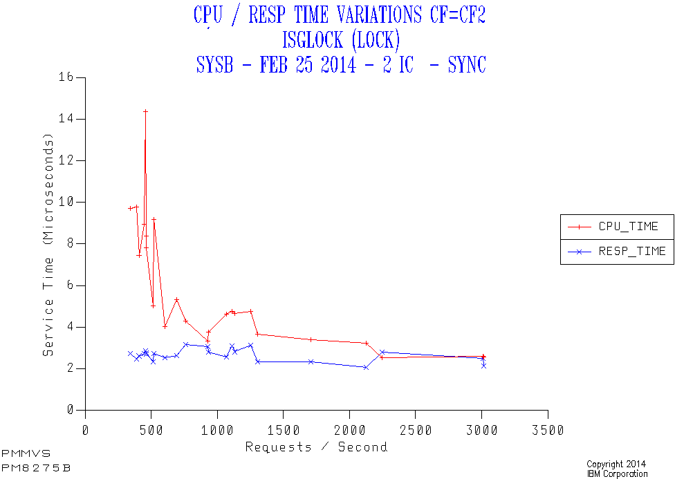
This is another lock structure (GRS Star instead of a DB2 LOCK1 structure). This time it’s in a different coupling facility (CF2) accessed through Internal Coupling (IC) links from the same member (SYSB).

Again all the requests are synchronous. But this time the response time is about 3 microseconds rather than the 10 for the first case. While the responsiveness to applications might not be very different there is an important effect:

Because all the requests are synchronous every request results in a coupled z/OS engine spinning for the entire duration of the request. For this reason the difference between 3 and 10 microseconds might well matter.

Obviously the further the distance and the slower the link technology the bigger the impact on request response times and, potentially the coupled CPU time.

Request CPU Heaviness

The two Lock Structure examples above had about the same CF CPU heaviness – 3 microseconds per request.

Consider the following case. It’s a DB2 Group Buffer Pool structure.

Here the CF CPU per request is variable but in the region of 15 to 20 microseconds, far heavier than for the two lock structures. As this structure is accessed from SYSB using IC links the CF CPU time dominates. So a slower CF engine would lead to longer request response times – under cirumstances like these where there is little CPU queuing in the CF.

(Notice how the Synchronous %[12] varies between 90% and 100% across the range of request rates. This could be a different mix of request types – as is entirely feasible with cache structures – or it could be the Dynamic Request Conversion heuristic converting some from Synchronous to Asynchronous as the response time increases. I prefer the former explanation here, but I’m not sure and no instrumentation will tell me.)

Conclusion

As always “it depends”. I’ve tried to give you a glimpse of on what and how it depends.[13] But usually I would expect a zBC12 stand alone coupling facility to be fine.

I appreciate that, if you’ve got this far, it’s been a very long read. Along the way you’ll’ve seen three graphs that each of them slightly “misbehave”: I consider the complexity and misbehaviour part of the deal when discussing Parallel Sysplex configuration and performance: It’d be hard to boil it down without missing something important.

 

(Originally posted 2014-03-23.)

I’m writing about intervals again.[1]

Two things have occasioned this:

• I’ve been updating my code for DB2 Versions 10 and 11[2].
• I’ve dealt recently with customers with unhelpful SMF or RMF intervals.

As I’ve said before it’s important to understand the provenance of the data you’re using. This would be true whether it’s performance data, financial data, health data or anything else.

Most of the time you don’t see raw data: It’s as processed as the food we eat. 🙂 I’m privileged[3] to spend more time than most looking at raw SMF records, though they too aren’t “the horse’s mouth” really.

DB2 Statistics Trace

DB2 Version 10 introduced a significant change in the way its interval-based records are created.[4] As previously noted STATIME governs the frequency with which Statistics Trace records are cut. The default dropped from a useless 30 minutes to 5 in DB2 Version 9. The change in Version 10 was to decouple the frequency of cutting certain types of Statistics Trace records from STATIME: IFCIDs 1, 2, 202, 217, 225 and 230 are always cut every minute. I use most of these IFCIDs (and rarely the ones that aren’t) so this is a good change for me.

But why do we care about the record-cutting interval? Let me take you on a journey from the raw SMF to the numbers I share with you (or which appear in any product’s reporting).

Consider the following spreadsheet and set of three graphs. It’s made up data but is typical of some of the counters in DB2 Statistics Trace.

Top left is the raw spreadsheet data:

• The first column is the record timestamp. Notice how the table is sorted by timestamp ascending.
• The second column is the raw field’s value. Notice how it is ever increasing.[5]

The remaining columns aren’t in the record but are derived:

• The third column is obtained by subtracting this record’s value for the field from the previous record’s. This is the delta in the spreadsheet and represents the activity in the interval.
• The final column is the delta converted to a rate: The interval here was 10 minutes or 900 seconds.

The result of all this is the graph on the bottom right (labelled (3)).

In reality I tend to summarise DB2 statistics by hour and all the data in the spreadsheet represents a single net data point. Also I take the lowest value in the interval (the first) and subtract from the highest (the last).[5] I suspect everyone else does too – after all a previous record just prior to the reporting period might not exist. But back to the data:

If you examine the time intervals covered 9:01 to 9:51 is only 50 minutes out of the hour. And the delta (19500–10000) covers those 50 minutes only. So the best rate calculation is 9500 / 3000 = 3.2 per second. In fact I do 9500 / 3600 and thus underestimate a fair bit.

It’s probably a little picky to also point out that the rate within the hour might significantly vary from this 3.2 figure because of surges or drops in activity outside the 50 minutes of the hour captured.

Actually a (simulated) STATIME of 10 (as in here) isn’t so bad: Losing some rate doesn’t matter much. But consider the old default of 30 minutes for STATIME: It’s highly likely 50% of the activity isn’t captured and that there is significant variation of rate outside of the 30 mins in the hour that is.

And that’s why I was so glad the default STATIME got dropped in Version 9. And why having these records cut every single minute in Version 10 is even better: Less than 2% of the activity and time is uncaptured – with a 1-minute interval.

RMF Intervals

Recently I’ve seen customers with long RMF intervals (1 hour) and with inconsistent intervals (30 minutes for some systems and 20 for others).

Both of these lead me to have to summarise data at an hourly level. I consider it a form of “enforced squinting”.[6]

Summarising at an hourly level makes the graphs more readable but, and this is a significant “but”, some peaks are shaved off. I’m most worried about underestimating[7] things like peak CPU busy. (Conversely overestimating WLM Service Class Period Velocity.) Both of these can lead to installations having a flawed capacity plan, with the potential for performance crises. Over the years I’ve seen my fair share of these.

It would be a bit much, most of the time, to lower the RMF interval down to, say, 1 minute. Benchmark or test run situations might be an exception but 1440 data points a day per system is excessive. 15 minutes is generally fine.

Of course processors (or engines if you prefer) are rather binary: At any moment an engine is either 100% busy or 0% busy. Zooming right in would yield this rather useless “whiplash” information.

I could, in principle, zoom out from the lowest level of summarisation – the RMF interval – to 1 hour, 2 hours, 4, 8, then 24 – to show how the average CPU Utilisation peaks at lower and lower values. And one day I just might: It’d be a good pedagogical exercise.

In the RMF case there’s no possibility of activity loss with long intervals, but there clearly is one of resolution loss.

It’s also helpful, by the way to synchronise the RMF interval with the SMF interval: Drilling down from the RMF Service Class Period level to the Address Space level works better if you do.

Data Volume Sensitivity

So, dropping the interval with which you cut records is a good thing, in data quality terms. But how is it in terms of quantity?

In the case of DB2 Statistics Trace the amount of data is dwarfed by the amount of Accounting Trace, assuming you’re collecting the latter. So a shorter interval probably doesn’t affect your overall SMF data volume significantly.

In the case of RMF there are some high-volume records, most notably SMF 74–1 (Device Activity), 74–5 and 74–8 (Cache), and 74–4 (Coupling Facility Activity). Unless you disable these types you’ll collect much more data if you drop the RMF interval significantly.

So, I like the current product behaviours – 1 minute for most of DB2 Statistics Trace and RMF’s default interval of 15 minutes – as a good balance between quality and quantity.

But essentially I’m after a decent interval. 🙂

(Originally posted 2014-03-15.)

As you know I mainly deal in SMF data (and other machine-generated instrumentation). While I’m perfectly adept at conducting interviews and handling evidence from real live people there’s much merit in instrumentation.

I’m also not keen on just replaying what you say back at you, with no value added in the process. But I’m making an exception:

I’ve just added to my code the ability to name physical processors or machines as I prefer to call them. That’s part of the origin of the title of this post.[1]

What RMF actually provides to label a physical processor is the plant number (eg “51”)[2] and serial number (eg “12345”). Previously I just printed this. In this example I would print “51–12345”. I think you’ll agree this isn’t a great way to refer to a machine. In fact not many customers are familiar with their machine serial numbers.

So, if you tell me the plant and serial number and what you call the machine I’ll use that information to build a table which my code uses to label graphs and reports. In fact if you say something like ’the System z10 with SYSA on is called “Ewelme A” or some such I can work it out from there.

So I’m reliant on two human factors here:

• You telling it to me straight.
• My not getting confused and building the table wrong.

I think I trust you to do your bit right more than me to do mine. 🙂

Actually my bit is fiddly: I wrote very simplistic code that literally takes plant and serial number and a name on a single line. It doesn’t take any other form of identification. So I have to use other means to correlate plant/serial and customer-friendly name.

As I said I’m not wowed at manually inputting anything. But in this limited case I think it’s worth it: I’d far rather use the terms (including pronunciation) you use, rather than an identifier you’ve never heard of. It just seems courteous and friendly. And as if the machine was a real one. 🙂

And of course, as most recently discussed in LPARs – What’s In A Name? I’m somewhat inquisitive about names anyway. 🙂

(Originally posted 2014-03-08.)

It’s only fair to warn you this gets technical straight away. And is probably only interesting to a DB2 audience anyway. And as someone who disclaims on his DB2 knowledge anyway you might not want to read this. 🙂

Still with me? Excellent!

As described in Coping With DB2 Version 10 And Preparing For DB2 Version 11 I’ve been revamping my DB2 analysis code.[1] Here are a couple of areas I think you might be interested in:

When Package And Plan Level Accounting Appear To Disagree

While I like to ensure my reporting matches that produced by IDMS products there is another kind of corroboration sensible reporting developers should try: Where possible check two data sources agree: For example DB2 Statistics Trace and DB2 Accounting Trace.[2]

This story relates to two different sections of the same record type:[3] The plan-level timings sections (QWAC and QWAX) appeared to disagree with the package-level[4] timing section (QPAC):

When you read the description of QWACAWTI it appears to be all the synchronous I/O time. A long time ago another field was introduced – QWACAWLG – which is the synchronous Log Write I/O time. This looked like a breakout of QWACAWTI and so I treated it that way.

The QPAC section also has a field like this called QPACAWTI. My DB2 Batch analysis code allows me to compare the plan- and package-level timings. So I discovered that – for specimen jobs – QWACAWTI was much less than the sum of all the QPACAWTI times. This didn’t make sense to me. Adding QWACAWLG to QWACAWTI got me the sum of the QPACAWTI times. Actually this does make sense as there is no package-level equivalent of QWACAWLG.

So now my code works properly – in this one regard.[5]

The byproduct is I know these jobs have substantial issues with logging speed: Either too much logging or too low logging bandwidth. Actually I do know which package has the logging issue in most cases as it’s the one with the big QPACAWTI value.

Row Count Statistics

This is a nicer story as it involves some newish statistics. In DB2 Version 9 Row Count statistics were introduced in the plan-level QXST section of Accounting Trace. In all likelihood you didn’t notice them. I certainly didn’t.

Let’s take one example: A basic statistic that’s been in the record forever is QXFETCH – the number of Fetch statements.[6] But one Fetch statement doesn’t necessarily equate to one row fetched. As someone who’s not in the habit of coding SQL I can immediately think of two scenarios where the two are different:

• In programs where you open a cursor you Fetch rows until there are no more rows available. The last Fetch statement doesn’t return a row.

• With the quite old now Multi-Row Fetch statement returns more than one row. This is for efficiency. Even returning two rows at a time is better than one, though changing to it is complex enough that you might want to return, say, 10.[7]

In both these cases the number of rows fetched is different from the number of Fetch statements and the new QXRWSFETCHD field could be compared to QXFETCH.

One possibility that immediately springs to mind is detecting when a program consistently finds no rows: That would seem unfortunate.

Another possible use is comparing the rows fetched by a program with the number of records written to a sequential data set (estimated from SMF Type 15 records).[8] That would help identify cases where the program is extracting records and directly writing them out.

While I’ve only talked about Fetch the same applies to Insert, Update and Delete. This doesn’t get us to omniscience with SMF but does give us some handy clues. While I haven’t finalised my design for reporting using these fields you can see it’s got me thinking.

---

So, as with all new data (or data I haven’t revisited in a while) I’m learning new tricks. And as I learn more I’ll continue to write about them.