(Originally posted 2019-08-02.)

(I’m indebted to Howard Hess for the title. You’ll see why it’s appropriate in a bit.)

Since I wrote Engineering – Part Two – Non-Integer Weights Are A Thing I’ve been on holiday and, refreshed, I’ve set to work on supporting the SMF 99 Subtype 14 record.

Working with this data is part of the original long-term plan for the “Engine-ering” project.

Recall (or, perhaps, note) the idea was to take CPU analysis down to the individual processor level. And this, it was hoped, would provide additional insights.[1]

Everything I’ve talked about so far – in any medium – has been based on one of two record types:

• SMF 70 Subtype 1 – for engine-level CPU busy numbers, as well as Polarisation and individual weights.
• SMF 113 Subtype 1 – for cache performance.

SMF 99 Subtype 14 provides information on home locations for an LPAR’s logical processors. It’s important to note that a logical processor can be dispatched on a different physical processor from its home processor, especially probably in the case of a Vertical Low (VL)[2]. I will refer to such things as where a logical processor’s home address is as “processor topology”.

It should be noted that SMF 99–14 is a cheap-to-collect, physically small record. One is cut every 5 minutes for each LPAR it’s enabled on.

Immediate Focus

Over the past two years a number of the “hot” situations my team has been involved in have involved customers reconfiguring their machines or LPARs in some ways. For example:

• Adding physical capacity
• Shifting weights between LPARs
• Varying logical processors on and off
• Having different LPARs have the dominant load at different times of day

All of these are entirely legitimate things to do but they stand to cause changes in the home chips (or cores) of logical processors.

The first step with 99–14 has been to explore ways of depicting the changing (or, for that matter, unchanging) processor topology.

I’ll admit I’m very much in “the babble phase”[3] with this, experimenting with the data and depictions.

So, here’s the first case where I’ve been able to detect changing topology.

Consider the following graph, which is very much zoomed in from 2 days of data – to just over an hour’s worth.

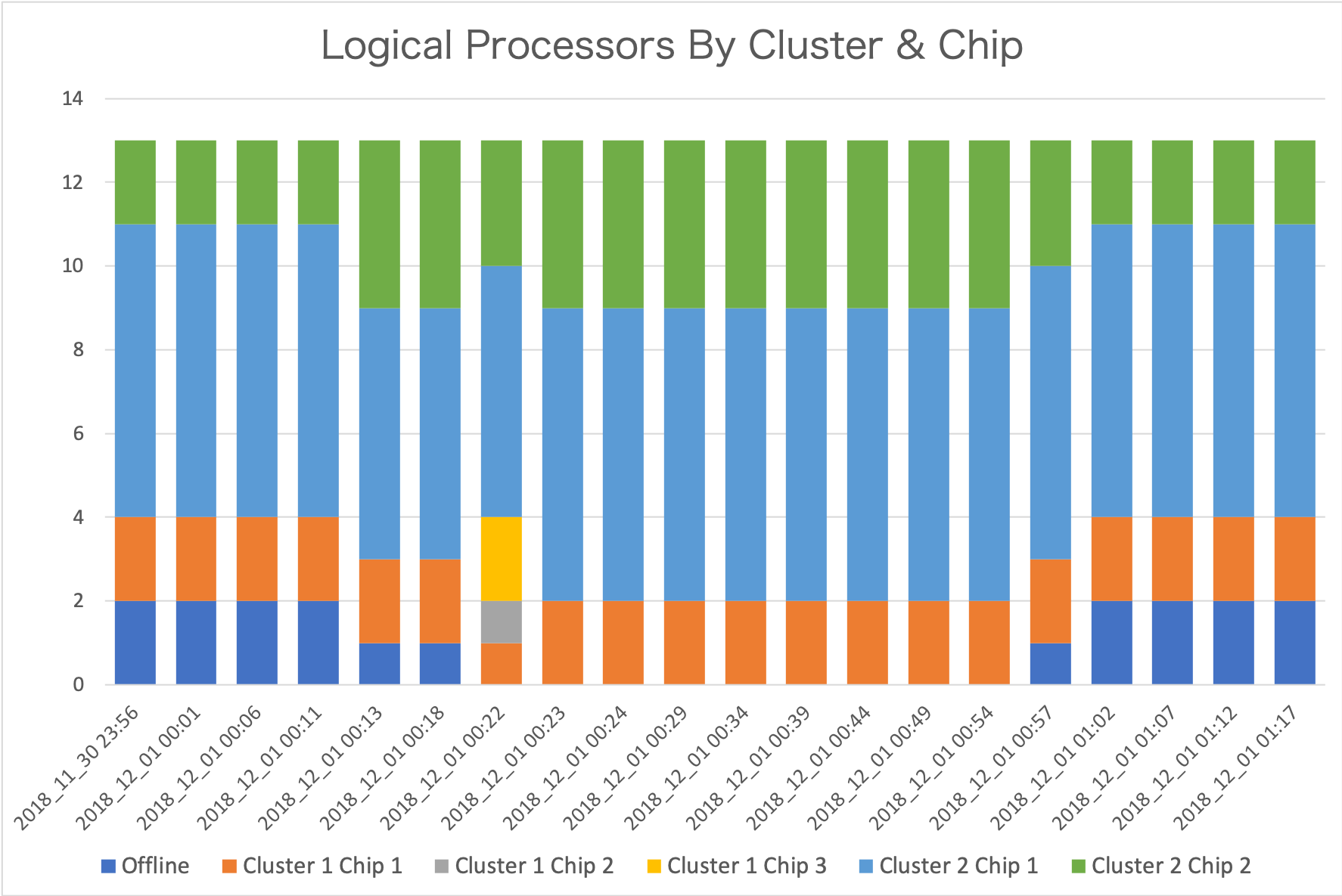
Each data point is from a separate record. From the timestamps you can see the interval is indeed 5 minutes. This is not the only set of intervals where change happens. But it’s the most active one.

There are 13 logical processors defined for this LPAR. All logical processors are in Drawer 2 (so I’ve elided “Drawer” for simplicity.)

Let me talk you through what I see.[4]

1. Initially two logical processors are offline. (These are in dark blue.) Cluster 2 Chip 1 has 7 logical processors and Cluster 2 Chip 2 has 2.
2. A change happens in the fifth interval. One logical processor is brought online. Now Cluster 2 Chip 1 has 6 and Cluster 2 Chip 2 has 4. Bringing one online is not enough to explain why Cluster 2 Chip 2 gained two, so one must’ve moved from Cluster 2 Chip 1.
3. In interval 7 another logical processor is brought online. The changes this time are more complex:
   • A logical processor is taken away from Cluster 1 Chip 1.
   • A logical processor appears on Cluster 1 Chip 2.
   • Two appear on Cluster 1 Chip 3.
   • One is taken away from Cluster 2 Chip 2.
4. Towards the end, as each of two logical processors are offlined they are taken away from Cluster 2 Chip 2.

The graph is quite a nice way of summarising the changes that have occurred, but it is insufficient.

It doesn’t tell me which logical processors moved.

What we know – not least from SMF 70–1 – is the LPAR’s processors are defined as:

• 0 – 8 General Purpose Processors (GCPs)
• 9 – 12 zIIPs

The Initial State

With 99–14, diagrams such as the following become possible:

This is the “original” chip assignment – for the first 4 intervals.

This is very similar to what the original WLM Topology Report Tool[5] would give you. (I claim no originality.)

I drew this diagram by hand; I can’t believe it would be that difficult for me to automate – so I probably will.[6]

After 1 Set Of Moves

Now let’s see what it looks like in Interval 5 – when a GCP was brought online:

GCP 5 has been brought online in Cluster 2 Chip 2, alongside the 2 (non-VL) zIIPs. But also GCP 0 has moved from Cluster 2 Chip 2 to Cluster 2 Chip 1.

What’s The Damage?[7]

Now, what is the interest here? I see two things worth noting:

• A processor brought online has empty Level 1 and Level 2 caches.
• A processor that has actually moved also has empty Level 1 and Level 2 caches.

Within the same node/cluster or drawer probably isn’t too bad. (And within a chip – which we can’t see – even less bad as it’s the same Level 3 cache). Further afield is worse.

Of course the effects are transitory – except in the case of VLs being dispatched all over the place all the time. Hence the desire to keep them parked – with no work running on them.

After The Second Set Of Moves

Finally, let’s look at what happened when the second offline GCP was brought online – in Interval 7:

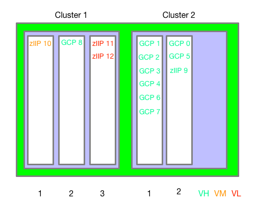
GCP 8 has been brought online in Cluster 1 Chip 2. But also zIIP 10 has moved from Cluster 2 Chip 2 to Cluster 1 Chip 1. Also zIIPs 11 and 12 have moved from Cluster 1 Chip 1 to Cluster 1 Chip 3.

This information alone (99–14) isn’t enough to tell you if there was any impact from these moves. However, you can see that in neither case was a “simple” varying a GCP online quite so simple. Both led to other logical cores moving. This might be news to you; It certainly is to me – though the possibility was always in the back of my mind.

Note: This isn’t a “war story” but rather using old customer data for testing and research. So there is no “oh dear” here.

Later On

To really understand how a machine is laid out and operating you need to consolidate the view across all the LPARs. This requires collecting SMF 99–14 from them all. This, in fact, is a motivator for collecting data from even the least interesting LPAR. (If its CPU usage is small you might not generally bother.)

But there’s a snag: Unlike SMF 70–1, the machine’s plant and serial number isn’t present in the SMF 99–14 record. So to form a machine-level view I have two choices:

• Input into the REXX exec a list of machines and their SMFIDs.
• Have code generate a list of machines and their SMFIDs.

I’ll probably do the former first, then the latter.

What also needs doing is figuring out how to display multiple LPARs in a sensible way. There is already a tool doing that. My point in replicating it would be to add animation – so when logical processors’ home chips change we can see that.

Maybe Never

SMF 99–14 records aren’t cut for non-z/OS LPARs, which is a significant limitation. So I can’t see a complete description of a machine. For that you probably need an LPAR dump which isn’t going to happen on a 5-minute interval.

However, for many customer machines, IFL- and ICF-using LPARs are on separate drawers. It’s a design aim for recent machines but isn’t always possible. For example, a single-drawer machine with IFLs and GCPs and zIIPs will see non-z/OS LPARs sharing the drawer. Most notably, this is what a z14 ZR1 is.

One other ambition I have is to drive down to the physical core level. On z14, for instance, the chip has 10 physical cores, though not all are customer-characterisable. But this won’t be possible unless the 99–14 is extended to include this information. This would be useful for the understanding of Level 1 and Level 2 cache behaviour.

Finally, there is no memory information in 99–14. I would dearly love some, of course.

Conclusion

While 99–14 doesn’t completely describe a machine, it does extend our understanding of its behaviour by relating z/OS logical processors to their home chips. Taken with 70–1 and 113–1, this is a rather nice set of information.

Which prompts lots of unanswerable questions. But isn’t that always the way? 🙂

A question you might have asked yourself is “do I need to know this much about my machine?” Generally the answer is probably “no”. But if you are troubleshooting performance or going deep on LPAR design you might well need to. Which is why people like myself (and the various other performance experts) might well be involved anyway. So – for us – the answer is “yes”.

The other time you might want to see this data “in action” is if you are wondering about the impact of reconfigurations – as the customer whose data I’ve shown ought to be. 99–14 won’t tell you about the impact but it might illuminate the other data (70–1 and 113). And together they enhance the story no end.

(Originally posted 2019-06-18.)

In Automation On Tap I talked about NFC tags and QR codes as ways of initiating automation.

This post is about a different initiator of automation.

I recently acquired the cheapest (and least functional) Elgato Stream Deck. This is a programmable array of buttons. My version has 6 buttons but you can buy one with 15 and one with 32 buttons.

A Previous Attempt Didn’t Push My Buttons

A while back I bought an external numeric keypad for my MacBook Pro. When I was editing our podcast with Audacity on the Mac I used this keypad to edit. It’s just numeric, with a few subsidiary keys.

What makes this programmable is that the Mac sees external keypad keys as distinct from their main-keyboard counterparts. So the “1” key on the external keypad has a different hardware code from the “1” key on the main keyboard. Keyboard Maestro macros can be triggered when keys are pressed. So I wrote macros to control Audacity, triggered by pressing keys on the external keypad.

But there was a problem: How do you know what each button does? It’s quite a pretty keypad – as you can see:

So I really didn’t want to stick labels on the key tops. I also tried to make my own template but there was an obvious difficulty: It’s hard to design one that tells you what the middle buttons in a cluster do.

There’s another problem: Suppose I set up automation for multiple apps – which Keyboard Maestro lets you do. Then I need a template for each app – as each will probably have its own key pad requirements. These templates are fragile and in any case this is a fiddly solution.

So this was good – up to a point. It certainly made podcast editing easier. But that was all.

And then I moved podcast editing to Ferrite on iOS, discussed here. And this keypad is now in a drawer. 😦

The One That I Want

Cue the Elgato Stream Deck Mini. First I should say there are other programmable keypads but this is the one that people talk about. I’d say with good reason.

As you can see, it’s corded and plugs into a USB A port.[1] Power to it is supplied by this cable.

It’s easy to set up, literally just plugging it in. To make it useful, though, you need their app – which is available for Mac or Windows. It’s a free app so no problem.

With their app you drag icons onto a grid that represents the Stream Deck’s buttons. Here’s what mine generally looks like when powered up and the Mac unlocked.

The key thing[2] to notice is the icons on the key tops. This is already a big advance on paper templates and ruined shiny key pads. I didn’t have to do anything to get these icons to show up[3]. What you can see is:

• 4 applications – Sublime Text, Drafts, Airmail and Firefox.
• A folder called “More”. More 🙂 on this in a moment.
• Omnifocus Today

The applications are straightforward, but the Omnifocus Today one is more complex. Pushing the button simulates a hot key – in this case Ctrl+Alt+Shift+Cmd+T. I’ve set up a Keyboard Maestro script triggered by this – extremely difficult to type – hot key combination. This script brings Omnifocus (my task manager) to the front and – via a couple of key presses – switches to my Today perspective.

So it’s not just launching applications. It can kick off more complex automation.

And someone built a bridge to IFTTT’s Maker Channel – which could open up quite a lot of automation possibilities. But right now I only have a test one – which emails me when I press the button.

One thing I haven’t tried yet is setting up buttons to open URLs in a browser. I don’t think I’ve got the real estate for that, with only six buttons.

Unreal Estate

In reality I probably should’ve plumped for the 15 button one[4], rather than the 6, but this has been an interesting exercise in dealing with limited button “real estate”.

So, if I press the “More” button I get this:

Because the button tops are “soft” they can change dynamically – as this demonstrates. This is much better than sticking labels on physical keys.

Two features of note:

• The back button – top left
• The “Still More” button bottom right

Being able to create the latter means I can nest folders within folders. This greatly increases my ability to define buttons.

The Right Profile

There’s one final trick that’s worth sharing.

Everything I’ve shown you so far has been from the Default Profile. You can set up different profiles for different apps.

I happen to have a few Keyboard Maestro macros for Excel – to make it a little less tedious to use. So I created a profile for Excel.

So when Excel is in the foreground the Stream Deck looks like this:

I’m still setting it up – and you can see two undefined (blank) buttons. – but you get the general idea. The two Excel-specific buttons – using an image I got off the web[5] – kick off some really quite complex AppleScript:

• Size Graph – which resizes the current Excel graph to a standard-for-me 20cm high and 30cm wide. This is fiddly so having a single button press to do it is rather nice.
• Save Graph – which fiddles with menus to get to the ability to save a graph as a .PNG file with a single button press.

(In retrospect I should probably have changed the text to black – which is easy to do.)

So in real estate terms, application-specific profiles are really handy.

One pro tip: Close the Stream Deck editor if you want application-specific profiles to work. I spent ages wondering why they didn’t – until I closed the editor.

Conclusion

This programmable key pad with dynamically-changing keytops is a really nice way to kick off automation from a single key press (or a few if you use cascading menus).

I would go for the most expensive one you can afford – but I’ve shown you ways you can get round the 6-button constraint in the Stream Deck Mini.

Application-specific profiles are a really nice touch.

The whole thing is rather fun for an inveterate tinkerer like me. 🙂

In short, I think I’ll be throwing this in my backpack and taking it with me wherever my MacBook Pro goes.

And one day I’ll upgrade to a model with more buttons.

(Originally posted 2019-06-18.)

You’ll have to pardon the pun in our latest podcast episode’s title.

We were also somewhat delayed in getting this out – due to our busy schedules and a few technical gremlins. Hopefully it’s worth the wait.

It’s also quite a long episode so if you listen to it on your commute you’ll have to ask your chauffeur to drive a little more slowly. 🙂

Episode 24 “Our Wurst Episode”

Here are the show notes for Episode 24 “Our Wurst Episode”. The show is called this because we both attended the IBM TechU in Berlin, Germany, and our Topics topic is our trip report.

Feedback

• We have some feedback (again) based on our use of stereo. We now have glorious mono, based on those comments!

Follow up

• We talked about smart thermostats in Episode 23, and a popular app, IFTTT . The API that allows IFTTT to monitor the Nest is going away on August 23, 2019.It is deprecated in favor of Google Home, with Google’s own Assistant routines Google Discontinues ‘Works With Nest’ Program, Tightens Smart Home Privacy Rules.

• These events just reinforces the view that – at least for now – automation is empheral.

What’s New

• APAR OA55959: NEW FUNCTION – PDUU Support for HTTPS
  • AMAPDUPL: Problem Documentation Upload Utility
  • How you get a dump to IBM, can be compressed, optionally encrypted, and sectioned into smaller data sets
  • HTTPS is important in this because dump can contain sensitive information and FTP is not an acceptable solution for many customers
  • FTPS had issues with e.g. firewalls,
  • Doesn’t look like this option has been incorporated into z/OSMF Incident Log at this time
• Tailored Fit Pricing for IBM Z
  • Enterprise Capacity Solution
  • Enterprise Consumption Solution
  • Both different from traditional rolling four hour average model
  • For Tailored Fit Pricing, all machines must be IBM z14 Models M01-M05 or ZR1, and at IBM z/OS V2.2, or higher
  • More information here.
  • In Episode 19 Performance topic we talked about Licence-Related Instrumentation.
• Ask MPT
  • Danny Naicker asks, “In z/OS 2.4 CSA subpool key 8–15, is it usable for user defined applications?”
  • Answer: Prior to z/OS V2.4 User Key Common Storage was available, but it was turned off by default. The downside was no control over who could use it.
    • In base V2.4 that specific capability has gone (the old system-wide switch).
    • Question probably originates from need to still use User-key CSA because of legacy stuff
    • This is where RUCSA (Restricted Use Common Service Area), a new function, comes into play. Allows you to identify applications by using a security definition.
    • Usage of RUCSA prior to V2.4 will need APAR OA56180
    • RUCSA will be offered in V2.4.
  • Thank you to Danny for a good question!

Mainframe Topic: CICS ServerPac in z/OSMF

• IBM’s first delivery on new installation strategy, will be with CICS and associated SREL products. This is the first of many (really, all).
• Choice on new installation strategy or old during ShopZ ordering. Choice is:
  • Old is ISPF CustomPac dialogs, or
  • New is z/OSMF Software Management and Workflows.
• We encourage making the z/OSMF choice, as that is consistent between IBM and other vendors, and is intended to be easier.
• Infrastructure already available in continuously delivery PTFs, and rolled back to z/OS V2.2. This makes the driving system have the proper infrastructure so anybody can package and deliver that way.
• More details on the z/OS installation strategy:
  • Software vendors will package similarly, in a z/OSMF Portable Software Instance,
  • Clients will be able to acquire and deploy and configure using z/OSMF.
  • z/OSMF Software Management is used to the acquisiting and deployment. (“Deployment” is the new term for “installation”!)
  • z/OSMF Workflows is used for configuration. You would see the old ServerPac batch jobs as steps in a Workflow.
• All software that you ordered as a ServerPac, and installed either way, will give you the same (or hopefully better) equivalent installation.
• There is an IBM Statement Of Direction that this installation choice is coming, but we do not have an exact date yet.
• For other software ISVs, they can exploit the new z/OS installation strategy whenever they are ready.
• Prepare now by becoming familiar with z/OSMF Software Management and Workflows
  • For Workflows, a short video might help. The sample Workflow used in this video you can start with has been moved here.
  • For z/OSMF Software Management screenshot paths, go here for software packaging, and here for software installation/deployment.

Performance Topic: DB2 And I/O Priority Queuing

• Follow on from Screencast / Blog post topic: Screencast 12 – Get WLM Set Up Right For DB2.
• Recent talk has been about whether to turn off I/O Priority Queuing in WLM.
• Service classes with DB2 subsystems in are heavily I/O Sample oriented, which is unusual among service classes in a system.
• Means access to CPU is not properly managed, as CPU & zIIP samples few, relative to I/O samples. Reminder: Most of DBM1 is now zIIP-eligible.
• Can achieve goal even with lots of delay for zIIP or CPU, but that’s definitely not what you want.
• To see if it is properly managed:
  • See if there are lots of CPU / zIIP Delay samples in RMF Workload Activity.
  • In Db2 might well see Prefetch etc engines exhausted, which could cause unwanted Sync I/Os and bad SQL performance.
    • The effect is just like if there is a real zIIP shortage.
  • Instrumentation for DB2 of relevance is Statistics Trace.
• You don’t want to just turn off WLM I/O Priority Queuing, as it’s sysplex-wide, it might affect other work that needs it, and Db2 might actually need it.
  • As the name suggests, it gives finer control over I/O priority.
  • So, it’s a case of proceeding with caution.
• First you need a reasonably achievable goal for the service class. Make sure you’re more or less achieving the existing goal.
• Second, calculate what the velocity achieved would be without I/O priority queuing .
  • Can take out the Using and Delay for I/O sample counts to do this.
• If you don’t do the analysis and act on it a shift to not using I/O Priority Queuing could have unpredictable results.
• You would know that turning off I/O Priority Queuing was helpful by seeing evidence that WLM is managing access to CPU for Db2 better, without hurting other stuff we care about. This evidence would come from RMF Workload Activity Report data.
  • On the Db2 side maybe Statistics Trace says Prefetch etc doesn’t get turned off. Or response times get better.
• You should evaluate or adjust the goal attainment, but that is BAU. Changing WLM always needs some care.

Topics: Berlin Trip Report May 20–24

• We both attended IBM Z TechU in Berlin, and got to see each other.
• Marna had about six sessions.
  • The SMP/E Rookies session had fabulous attendance – 44. Some were more experienced, but most were not.
  • z/OSMF had good attendance too, about 82. More are interested in this topic, especially if you compare to just a couple of years ago.
  • Best attended was the z/OS V2.4 Preview, with about 150 people. There was excellent interest in what is coming in the new release.
• Marna got to do a couple of things outside the conference:
  • Visiting the Reichstag was fabulous, but make sure to get a reservation.
  • Der Dom was also educational, with a walk to the top!
• Marna did her own poster to help with z/OSMF configuration, and several people came by to chat.
• Both Marna and Martin shared a poster about this podcast. We helped with getting one person a podcast app (on each platform), and a subscription to this podcast.
• Martin had five sessions.
  • Two were with Anna Shugol, Engine-ering, and zHyperLink.
  • One was co-written with Anna, “2 / 4 LPARs”
  • Two were solo efforts: Parallel Sysplex Performance Topics, and Even More Fun With DDF
• Martin also took a little time out of the conference
  • Each day took a session out to walk in the city.
  • It was interesting to wander round former East Berlin.
• The next European IBM Z TechU is in Amsterdam May 25–29, 2020.

Customer requirements

• RFE 131187
  • zOSMF RESTFILES PUT to remove Windows Carriage Return characters
  • Windows files contain a carriage return and line feed and the carriage return character x’0D’ is not being removed. The resulting zOS datasets therefore have a blank line after every data line that shouldn’t be there.

Future conferences where we’ll be

• Both Marna and Martin in SHARE, Pittsburgh, August 5–9, 2019

On the blog

• Martin has several blog posts:
  • Engineering – Part Zero
  • Engineering – Part One – A Happy Medium?
  • Engineering – Part Two – Non-Integer Weights Are A Thing
  • What’s In A Name? – Revisited Again
  • A Slice Of PI
  • Elementary My Dear Sherlock
• Marna has one, which the Mainframe topic was based on:
  • z/OS CICS ServerPac in a Portable Software Instance Planned

Contacting Us

You can reach Marna on Twitter as mwalle and by email.

You can reach Martin on Twitter as martinpacker and by email.

Or you can leave a comment below. So it goes…

(Originally posted 2019-06-08.)

Students of English literature won’t be alone in recognising the allusion in this post’s title.But this post isn’t about literature.[1].

Sherlocking, as described here is a phenomenon where a developer ships something – typically an app – but then Apple comes along and announces its own version of it.

In very recent memory, examples might be:

• Enhancements to Apple’s Reminders apps on iOS and Mac OS versus Omnifocus and other “to do list” apps – in iOS 13 and Mac OS 10.15 Catalina.
• NFC tags kicking off Apple Shortcuts automation versus LaunchCenter Pro’s support of NFC tags (described in Automation On Tap) – in iOS 13.
• Apple Watch Calculator and PCalc – in Watch OS 6.

But what of it?

At first sight, having your app Sherlocked must be disheartening. But that’s not the end of the story.

What’s at risk for the vendor that gets Sherlocked is subscriptions and future sales. In other words, revenue. For some apps – particularly those that don’t use a subscription model – the sales pattern might be that most sales happen early in the app’s life. So before Sherlocking happens.

But it’s not that simple. Yes, Sherlocking represents a threat but it also represents an opportunity…

… A platform vendor legitimizes a marketplace by sensitising users to the value of a function. For example the new Watch OS Calculator app will introduce users to the idea of a calculator on their wrist.[2] But if PCalc were a better calculator than the Apple one it could still sell well. Fortunately it is. 😁

A built-in app gives one you have to buy a run for its money and free beats fee for many customers – if the basic function is good enough.

But the built-in (Sherlocking) app is usually relatively basic so a purchased app wins by differentiation from the basic. So the message is Sherlocked apps must up their game.

(For me, while I wouldn’t want to wear the “Power User” badge the basic function is rarely good enough. For example I use the excellent Overcast podcasting app instead of the Apple one and it’s inconceivable I wouldn’t use it and hardly conceivable I wouldn’t pay for the premium version.)

Having said that, first party apps have some additional opportunities for integration so could have some advantages. It’s difficult to compete against that. There are private APIs that only Apple can use – but those tend to open up over time.

Basic infrastructure – for example the Reminders database – done right allows third parties to use the infrastructure. Reminders data is shareable across platforms and with other third party apps designed to take advantage of the database.

A good example of a third party app using the Reminders database is Goodtask. Goodtask illustrates one downside of using the built in database, however: The developers had to use a lot of ingenuity to get round the limitations of the Reminders database: As they articulate here they use the Notes field for a task and had to invent their own metadata format.

Unfortunately Mail on iOS doesn’t have this open database and nor does Music.So email apps have to use their own databases – which is a real shame. It means, for instance, you can’t operate on the same email account with a mix of built-in and third party app functions. With Reminders and Goodtask you can.

Here’s an example of why I would want Mail to be open: My favourite email client – on Mac and iOS – is Airmail. I favour it because it has more automation hooks than the default Mail app. But I can’t use it with my work email account because it doesn’t share the default Mail app’s database.

Automation is one area where Apple – as the platform vendor – has an advantage. Those of us who are into automation are still waiting for better automation than x-callback-url[3] – as Shortcuts doesn’t provide a general automation mechanism for third-party apps. A more general mechanism would certainly help. But I digress.

In summary, Sherlocking does represent a threat but also an opportunity. The way to make it the latter is for Sherlocked app developers to continually innovate – to differentiate their apps from Apple’s. Thankfully the best developers are fleet of foot; I don’t envy their position but the best will survive.

If they do innovate at speed the net is the consumer benefits.

(Originally posted 2019-06-01.)

A rather obscure pun, but I hope it’ll make sense. Not “Pi” by the way but “PI”. Though this post contains arithmetic, it’s not a mathematics post.

To be honest, I never knew how we calculated Performance Index (or PI) for Percentile goals before. But now I do, so I’m sharing it with you. Plus a couple of observations, too.

To be even more honest, when I say “I never knew how we calculated Performance Index” I should say “I never knew how we should calculate Performance Index” – as I’ve just corrected it.

(This post follows on (after 6 years) from WLM Response Time Distribution Reporting With RMF. More on that later.)

Before we go any further I have to give a little background information.

What Are Percentile Goals?

When Workload Manager (WLM) manages transactions explicitly two kinds of goals become available:

• Average Response Time
• Percentile

By the way, for WLM to manage transactions at all requires cooperation / exploitation by middleware or at any rate a work manager. Examples include:

• CICS transactions require CICS support
• DDF transactions require Db2 support
• TSO uses the traditional transaction ending mechanism
• Likewise Batch job steps

Average response time goals say something like “the average response time for this service class period should be 0.5 seconds”.

A Percentile response time goal might be “90% of all transactions in this service class period should finish in 300 milliseconds”.

What Is Performance Index – Or PI?

Performance Index (PI) is a measure of goal attainment.

• A PI of 1.0 is where the goal is just met.
• Higher than 1.0 and it is missed, the further away from 1.0 the worse the miss.
• Lower than 1.0 and it is met, the lower the greater ease in meeting the goal.

The point about PI is that it is a metric for goal attainment that is neutral with regard to workload type.

PI is, of course, used to drive WLM’s algorithms. But I regard it as just the first metric. Others, such as WLM’s ability to help a service class period, are important too.

How Do We Calculate PI For Percentile Goals?

The calculation for goal attainment for Average response time goals is straightforward: Sum up the response times for each transaction and divide by the number of transactions ending.

The calculation for Percentile goals is more complex.

For any kind of transaction-based goal, at transaction ending WLM uses the transaction’s response time to assign it to one of 14 buckets. So WLM is counting transaction endings in these buckets.

The buckets have the following boundaries:

The bolded values are of special significance, as we shall see.

Suppose we have a goal of “85% to complete within 0.2 seconds”. WLM knows how many transactions completed in each bucket and how many overall.

Suppose 1000 transactions completed. 85% of 1000 is 850 transactions.

Starting with Bucket 1, WLM tallies up the transaction endings until it meets 850 transactions. The upper limit of the bucket in which that happens is what determines the PI.

Suppose Buckets 1 to 3 tally up to 800 transactions and Bucket 4 contains 100 transactions. So Buckets 1 to 3 don’t meet 850 but Buckets 1 to 4 do.

Bucket 4’s upper limit is 80% of goal. So the PI is 80%/100 or 0.8.

Suppose it took Buckets 1 to 8 to reach or exceed 850. Then Bucket 7’s upper limit would be 110% and the PI would be 110%/100 or 1.1.

The code I inherited[1] didn’t do this calculation. But now it does.

Actually the calculation is not quite that simple: If by the time we’ve tallied up buckets 1 to 13 and we still haven’t reached that 850 number we set the PI to 4.0 (which makes sense).

Some Observations

From the above description of how PI is calculated for percentile goals, we can observe a few things:

• PI can never be greater than 4.0, no matter how widely the goal is missed.

• PI can never be less than 0.5 – as Bucket 1’s maximum is 50% of goal.

• A PI of 0.5 is special in that it means enough transactions ended in Bucket 1, and some could be much shorter than 50% of goal. To get further definition we’d have to calculate the average response time.

  Now I calculate PI right I’m seeing 0.5 quite a bit.

• If there are no transaction endings automatically the percentile goal is reached in Bucket 1 as all zero transactions ended there. So PI is meaningless with no transaction endings. so I force the PI to 0, but attempt to flag why in my reporting.

• Because we’re using buckets there are only a finite number of values PI can take. Averaging over multiple RMF intervals will, of course, yield more.

Revisiting That Old Blog Post

This seems as good a place as any to follow up on WLM Response Time Distribution Reporting With RMF.

I made some refinements to the graph I showed there:

• In the post I alluded to “near misses” versus “missed by miles” – and the counterpart on the “hits” side. I did indeed define “near” as +20% (and –20%) so Buckets 7–8 (and Buckets 5–6).
• I added a green datum line for the % value in the goal.
• I also added transaction rate. My code attempts to scale so that transaction rate doesn’t look ridiculous on a 0 to 100 scale.
• I considered changing from a red-through-to-green spectrum but I think that’s less consumable. Besides, I like red/blue better.

Here is a modern case of a CICS transaction service class.

Here are some observations:

• The datum is 95% because the goal is “95% in 1 second, Importance 1”.
• A goal with “1 second” in it suggests pretty heavy CICS transactions. I’m not surprised there aren’t that many transaction endings.
• When the transaction rate is significant the red pokes down below the green datum. Not just the pale red (“Just Outside”) but the darker red (“Well Outside”). You could say the blue shrinks away from it, if you prefer.
• Not shown here but the PI is typically around 1.3.

By the way, WLM doesn’t have complete control over the response time achieved for a transaction. And that’s particularly relevant here.

This transaction goal service class is served by two region goal service classes. Both of these show almost no “Delay For X” samples. What they do have is lots of “Using I/O” and “Using CPU” samples.

So, to improve transaction response time it’s probably necessary to try:

• Cutting the transaction CPU path length.
• Reducing the I/O time by (and this is only an example) buffering the data better.

Neither of these are things WLM can do[2].

(Originally posted 2019-05-27.)

It seems to be in the nature of my code development work that I revisit things over and over again. You could call it “agile”, you could call it “fragile”. 🙂 I prefer to think of it as being inspired by each fresh set of customer data.

And so it is with data set names. In What’s In A Name? – Revisited I talked about gleaning information from a data set name and using bolding to aid comprehension. This is an update to that, based on some new code.

But first a confession: I reopened this code because there was a bug in it. But while I was there I was inspired to capture another hill.[1] The very same dataset that caused my REXX to terminate with an error caused a nice piece of inspiration.

The Bad

The bug was in not recognising a Generation Data Group (GDG) data set could have “19” in its low-level qualifier. That led to misinterpreting the generation number as part of a date. (GDS low level qualifiers are of the form GnnnnVmm where the first variable part is the generation number and the second the version number – so “G1719V00” means “generation 1719, version 0”.)

That was an easy one to fix but on to the nicer part.

The Good

The data set name had “BKUP” as the last but one qualifier. This to my eyes signifies the data set is a backup for something. So I added a test to detect either “BKUP” or “BACK” in a qualifier and bold it if present.

I’ve made the code general enough so I can add further mnemonics – such as “OFFSITE” or “UNLOAD”. (In fact – since writing this post on the plane to Berlin I added full-qualifier matching for “OUT” and “NEW” as one of our job dossiers had data sets with these qualifiers.)

When I examine the data set names for one step in particular, every data set with “BKUP” as the low-level qualifier has a corresponding data set with an identical name, apart from the “BKUP” low-level qualifier being missing. The “BKUP” data set is an output data set (and I know about it because of its SMF Type 15 record). The matching data set is an input data set (and I know about it because of its SMF Type 14 record).

So I think we know what’s going on here[2]. 🙂

As I concluded in What’s In A Name? – Revisited there’s value in decoding data set names. And the more common gleanings I can do the better. This is just a nice little further step in that direction.

But I remain conscious of the possibility one could go too far, or get it wrong:

• Not every word in the English language that appears inside a data set name is significant.
• Not every significant word in a data set name is even English.

But we roll on. And no doubt the next study will bring fresh ideas for code. And that’s just the way I like it.

(Originally posted 2019-05-26.)

Maybe you’ve never thought much about this but aren’t weights supposed to be integer?

Well, they are at the LPAR level. But what about at the engine level?

Let me take you through a recent customer example. The names are changed but the numbers are real, as the one graphic in this post will show. The customer has a z14 ZR1 with 3 general-purpose processors (GCPs). The weights add up to 1000. Nice and tidy. There are two LPARs:

• PROD – with 3 logical engines and a weight of 965.
• TEST with 2 logical engines and a weight of 35.

Both LPARs are in HiperDispatch mode – which means the logical engines are vertically polarised.

To proceed any further we need to work out what a full engine’s worth of weight is: It’s 1000 / 3 = 333.3 recurring. Clearly not an integer. How do you assign vertical weights given that?

Let’s take the easy case first:

TEST has a weight of 35. Much less than one engine’s worth of weight. It has two logical processors so we would expect:

• A Vertical Medium (VM) with a weight of 35.
• A Vertical Low (VL) with a weight of 0.

So, in this case, both the engines have integer weights. So far so good.

Now let’s take the case of PROD. Here’s what I expect:

• Two Vertical Highs (VHs) each with a weight of 333.3 recurring. Total 666.6 recurring.
• A Vertical Medium (VM) with weight 965 – 666.6 recurring or 288.3 recurring. (It’s the presence of the non-integer VH’s that forces the VM to be non-integer.)
• No Vertical Lows (VLs).

When I say “expect” I really mean “what I’ve come to expect”. And I say that because I’ve seen it in reports produced by my code – and ended up wondering if my code was wrong. With the “Engine-ering” initiative, and in general because of HiperDispatch, it’s become more important to understand what’s going on at the logical engine level.

Non-integer weights began to worry me. So I started to investigate. Here’s the process, in strict step order:

1. My REXX code correctly queries my database at a summary table level and reports what it sees.
2. My database code correctly summarises the log level table.
3. My log level table correctly maps the record.

Let’s take a closer look at the record, which is what I did to establish Point 3.

When I look at individual records at the bits-and-bytes level I generally use RMF’s ERBSCAN and ERBSHOW execs:

1. If you type ERBSCAN against an SMF data set in ISPF 3.4 you get a list of records, each of which has a record number associated with it. Among other things the ERBSCAN list shows SMFID, timestamp and record type and subtype.
2. If you type ERBSHOW nnn where nnn is the number of an RMF record you get a formatted hex display of the record.

I emphasise RMF because ERBSHOW does a good job on RMF records, but no so useful a job for most other record types. (SMF 99-14 is one where I’ve seen it do a good job, but I digress.)

Anyway, back to the point., Here’s part of an ERBSHOW for an SMF 70-1 record. It shows five Logical Processor Data Sections – the first 3 for PROD and the last 2 for TEST.

The highlighted field is SMF70POW – the engine’s vertical weight. Here’s the full description of the 4-byte binary field:

Polarisation weight for the logical CPU when HiperDispatch mode is active. See bit 2 of SMF70PFL. Multiplied by a factor of 4096 for more granularity. The value may be the same or different for all shared CPUs of type SMF70CIX. This is an accumulated value. Divide by the number of Dignoase samples (SMF70DSA) to get average weight value for the interval.

So the samples are multiplied by 4096. Now 4096 is 1000 hexadecimal. So an integer would end with three hex zeroes, wouldn’t it? The first three clearly don’t.

But lets take the simpler – TEST – case first.

• SMF70DSA is 90 decimal.
• Section 4 has hex 00C4E000.Dividing by hex 1000 and converting to decimal we get 3150. Divide that by 90 and we get 35. So this is the VM mentioned above.
• Section 5 has zero so that is a vertical weight of 0. So this is the VL mentioned above.

Now let’s look at PROD.

• Each of the first two logical engines has SMF70POW of hex 0752FFE2. Clearly dividing by 1000 hex doesn’t yield an integer – so I (and my code) divide by SMF70DSA first. I get hex 0014D555 or decimal 1365333. Divide this by 4096 and I get 333.3 recurring.
• The third engine has SMF70POW of hex 068E203C. Divide by SMF70DSA and convert to decimal and I get 1221974 decimal. (Already this is less than 1365333.) Divide by 4096 and I get 298.3 recurring.

So my code is vindicated. Phew!

My suspicion is that vertical weights are held (not just sampled) multiplied by 4096.

But in any case the message is if the data looks odd then dig into it. In my case I blamed my own tools first but my tools are vindicated. But my expectation was wrong or, more charitably, blurry.

And, the more I think about it, the more the actual engine-level weights make sense. They have to add up to the LPAR weight. And the existence of Vertical Highs forces the above arithmetic on us.

But half the point of this post is to show how I debug numbers (and names) in my reporting that don’t meet my expectation. And ERBSCAN / ERBSHOW is a pair of friends you might like to get to know.

(Originally posted 2019-05-25.)

In Engineering – Part Zero I talked about the presentation that Anna Shugol and I have put together. That post described the general sweep of what we’re doing.

This post, however, is more specific. It’s about Vertical Medium logical processors.

To keep it (relatively) simple I’m describing a single processor pool. For example, the zIIP Pool. Everything here can be generalized, though it’s best to treat each processor pool separately.

Also note I use the term “engine” quite a lot. It’s synonymous with processor.

What Is A Vertical Medium?

Before HiperDispatch an LPAR’s weight was distributed evenly across all its online logical processors. So, for a 2-processor LPAR with weights sufficient for 1.2 processors, each logical processor would have 0.6 engines’ worth of weight.

Now let’s turn to HiperDispatch (which is all there is nowadays)¹.

The concept of A Processor’s Worth Of Weight is an important one, especially when we’re talking about HiperDispatch. Let’s take a simple example:

Suppose a machine has 10 physical processors and the LPARs’ weights add up to 1000². In this case an engine’s worth of weight is 100.

In that scenario, suppose an LPAR has weight 300 and 4 logical processors. Straightforwardly, the logical processors are:

• 3 logical engines, each with a full engine’s worth of weight. These are called Vertical Highs (VH for short). These use up all the LPAR’s weight.
• 1 local engine, with zero weight. This is called a Vertical Low (or VL).

There are a few “corner cases” with Vertical Mediums, but let me give you a simple case. Suppose the LPAR, still with 4 logical processors, has weight 270. Now we get:

• 2 VH logical engines, each with a full engine’s worth of weight. This leaves 70 to distribute.
• 1 logical engine, with a weight of 70. This is not a full engine’s weight. So this kind of logical processor is called a Vertical Medium (or VM).
• 1 VL logical engine, with zero weight.

Note that the VM in this case has 70% of an engine’s worth of weight.

How Do Vertical Mediums Behave?

There are two parts to HiperDispatch:

• Vertical CPU Management
• Dispatcher Affinity

Vertical CPU Management

Let’s take the three types of vertically polarized engines:

• With a VH the picture is clear: The logical processor is tied to a specific physical processor. It is, in effect, quasi-dedicated. The benefit of this is good cache reuse – as no other logical engine can be dispatched on the physical engine. Conversely, the logical engine won’t move to a different physical engine (leaving its cache entries behind).

• With a VM there is a fair attempt to dispatch a logical engine consistently on the same physical engine. But it’s less clear cut that this will always succeed than in the VH case. Remember a VM will probably be competing with other LPARs for the physical engine. So it could very well lose cache effectiveness.

• With a VL, the logical engine could be dispatched anywhere. Here the likelihood of high cache effectiveness is reduced.

The cache effects of the three cases are quite different: It would be reasonable to suppose that a VH would have better cacheing than a VM, which in turn would do better than a VL. I say “reasonable to suppose” as the picture is dynamic and might not always turn out that way.

But you can see that LPAR design – in terms of weights and online processors – is key to cache effectiveness.

We prefer not to run work on VLs – so the notion of parking applies to VLs. This means not directing work to a parked VL. VLs can be parked and unparked to handle varying workload and system conditions.

Dispatcher Affinity

With Dispatcher Affinity, work is dynamically subdivided into queues for affinity nodes. An affinity node comprises a few logical engines of a given type. Occasionally work is rebalanced.

You could, for queuing purposes, view an LPAR as a collection of smaller units – affinity nodes – though it’s not as simple as that. But that could introduce imbalance, a good motivation for the rebalancing of work I just mentioned.

What Dispatcher Affinity means is that work isn’t necessarily spread across all logical processors.

How Do They Really Behave?

With VMs I have three interesting cases, two of which I have data for. They got me thinking.

• Client A has an LPAR with 4 logical zIIPs. One is a VH, one is a VM with weight equivalent to 95% of an engine, and two are VLs. Here it was notable that there was reluctance to send work to the VLs – as one might expect. The surprise was that the VM was consistently loaded about 50% as much as the VH. For some reason there’s reluctance to send work there as well, but not as bad as to the VLs. The net effect – and why I care – is because the VH was loaded heavier than we would recommend, because of this skew.
• Client B has two LPARs on a 3-way GCP-only machine. One has two VHs and one VM with almost a whole engine’s worth of weight. In this case the load was pretty even across the 3 logical engines, according to RMF.
• Client C – for whom I don’t have data – are concerned because it is inevitable they’ll end up with 1 almost-VH logical engine.

So there’s some variability in behaviour. But that’s consistent with every customer environment being different.

Conclusion – Or Should We Avoid Vertical Mediums?

First, in many cases, there’s an inevitability about VMs, particularly for small LPARs or where there are more LPARs than physical engines. I’ll leave it as an exercise for the reader to figure out why every LPAR has to have at least one VH or VM in every pool in which it participates.

I don’t believe it makes any difference in logical placement terms whether a VM has 60% of an engine’s worth of weight or 95%. But I do think a 60% VM is more likely to lose the physical in favour of another LPAR’s logical engine than a 95% VM.

I do think it’s best to take care with the weights to ensure you don’t just miss a logical engine being a VH.

This thinking about Vertical Mediums suggests to me it’s useful to measure utilisation at the engine level – to check for skew. After all you wouldn’t want to have Delay For zIIP just because of skew – when the pool isn’t that busy.

But, of course, LPAR Design is a complex topic. So I would expect to be writing about it some more.

(Originally posted 2019-03-22.)

I’m writing this on a plane, heading to Copenhagen. Planes, like weekends, give me time to think. Or something. 🙂

Ardent followers of this blog will probably wonder why there have been few “original content” posts to this blog¹ recently.

Well, I’ve been working on an exciting project with my friend and colleague Anna Shugol. Now is the time to begin to reveal what we’ve been working on. We call this project “Engine-ering”².

The idea is simple: There is real merit in examining CPU at the individual processor level, for example the individual zIIP. As one colloquial term for processor is “engine” it’s easy to end up with a title such as “Engine-ering” and the hashtag #EngineeringWorks is way too tempting not to deploy.

The project has three parts:

• Writing some analysis code.
• Deploying the code into real customer situations.
• Writing a presentation.

These three are intertwined, of course. As we go on we will:

• Write more code.
• Gain more experience with it in customer situations.
• Evolve our presentation.

You’d expect nothing less from us.

Traditional CPU Analysis

Traditionally, CPU has been looked at from a number of perspectives:

• Machine and LPAR – with SMF 70-1.
• Workload and service class – with SMF 72-3.
• Address space – with SMF 30-2/3, also 4/5.
• DB2 transaction – with SMF 101 – and its analogues for other middleware.
• Coupling Facility – with SMF 74-4.

All of these have tremendous merit – and I’ve worked with them extensively over the years.

z/OS Engine Level

Our idea is that there is merit in diving below the LPAR level, even below the processor pool level. So we would want to, for example, examine the zIIP picture for an LPAR. But we wouldn’t want to just look at in in aggregate. We want to see individual processors. There are at least a couple of reasons:

• Skew between engines could be important.
• Behaviours, such as HiperDispatch parking, get thrown into sharp relief.

RMF

RMF (SMF 70-1) reports individual engines at two levels:

• This z/OS image.
• All the LPARs on this machine.

The trick is marrying these two perspectives together. Fortunately, a few years ago, I realised I could use the partition number of the reporting system and match it to the partition number of one of the LPARs. That does the trick.

In the past week I wrote some code to pump out engine level statistics for the reporting LPAR:

• Vertical weights
• Engine-level CPU utilization
• Parked (or unmarked) time

The first two are from the PR/SM view. The third is from the z/OS view. Which makes sense.

In any case I have some pretty graphs. And I got to swear at Excel a lot.³

SMF 113 Hardware Counters

This one is more Anna’s province than mine. But, processing SMF 113-1 records at the individual engine level, we now can see Individual engine behaviours in the following areas:

• We can see instructions executed, cycles used to execute them, and hence compute Cycles Per Instruction (CPI).
  


  At the individual engine level there is some very interesting structure, especially between Vertical Low processors (with zero vertical weight) and Vertical Highs (VHs) and Mediums (VMs).

  


  Actually there is a lot of difference sometimes between individual VH and VM engines.

• We can see the impact of Level 1 Cache misses – in terms of penalty cycles per instruction – for Data Cache and Instruction Cache individually. This begins to explain the CPI behaviors we see.
  


  Pro Tip: Understanding the cache hierarchy in a processor really helps, and it’s different from generation to generation.

Those of you who know SMF 113 know there are many more counters. We intend to extend our code to look at those soon.

SMF 99-12 And -14

Another area we intend to extend our code to analyse is SMF 99 subtypes 12 and 14. This data will tell us how logical engines relate to physical engines, right down to which drawer they’re in, which cluster (or node for z13), even which chip. All of this can help with understanding the “why” of what SMF 113 is telling us.

Coupling Facility

You can play a similar RMF-level game for coupling facilities. Normally, you wouldn’t expect much skew between CF engines. But in Getting Nosy With Coupling Facility Engines I showed this wasn’t always the case.

I would say that, while the “don’t run your coupling facility CPU more than 50% busy” rule is sensible you might want to adjust it for any skew your coupling facilities are exhibiting.

Outro

We presented this material the other day to the zCMPA working group of GSE UK. This was to a small number of sophisticated customers, most of whom I’ve known for many years. It’s become a bit of a tradition to present an “alpha” version of the presentation.⁴

This post roughly follows the structure of the presentation. In this presentation we have some very pretty graphs. 🙂

Anna coined the term “research project”. I like it a lot.⁵ In any case, the code is a permanent part of our kitbag. If you send me data, expect me to ask for this new stuff and to use it in conversations with you. I think you’ll enjoy it.

We think the presentation went very well, with some nice discussion from the participants. Partly because of that, but not really, we intend to keep capturing hills with the code, gaining experience with customers, and evolving the presentation. Every so often I’ll highlight bits of it here. Stay tuned!

(Originally posted 2019-02-27.)

This episode is hot on the heels of the previous one.

Marna set us the ambitious goal of getting it out on the day of the Preview Announcement of z/OS 2.4 – February 26th. And we succeeded. Phew!

I’m really excited about the Docker / Container Extensions (zCX) line item and I’m sure we’ll return to it – both as Mainframe and as Performance topics. Obviously, this being a Preview, that will have to wait a while.

So, I finally caved and mixed this Mono. I had no idea how I was going to do that. I hope y’all think it turned out OK.

I’m aiming to return to regular blogging soon. Right now there are things that I want to talk about but now is not quite the right time.

In the meantime, I hope you enjoy the show, and here are the notes.

Episode 23 “The Preview That We Do”

Here are the show notes for Episode 23 “The Preview That We Do”. The show is called this because we talk about the newly previewed z/OS release, V2.4, in the Mainframe section. This is our 24th episode too! How convenient! This episode is somewhat shorter than others because we wanted to slot it in for a particular date (the z/OS V2.4 Preview date) and we’d just done Episode 22.

Mainframe: z/OS V2.4 Preview

1. “z/OS Container Extensions” aka zCX

   • Intended to enable users to deploy and execute Linux on IBM Z Docker containers on z/OS. Not just run but also to enable application developers to develop and package popular open source containers.
   • It is clear that Docker is becoming prevalent with users. Now, z/OS could leverage industry standard skills, quickly on z/OS.
   • One could pull IBM Z Linux containers from Dockerhub. Latest count was 1724 in 14 categories.
   • Martin is interested in the instrumentation, and in the SMF records. Configuration we’ll cover in a future podcast.
   • The planned preqs for zCX are: z14 GA2 or higher, and will require a HW feature code
   • zCX is planned to be zIIP eligible.

2. z/OS Upgrade Workflow, no book

   • ”Upgrade” is the new term instead of ”Migration”
   • No z/OS Migration book, use the workflow instead. That requires you to become familiar with z/OSMF and workflows in particular.
   • Not everybody is familiar with z/OSMF, so we’ll export a workflow file and put it on Knowledge Center so you can view, search, print. However, the Workflow should give you a better experience.

3. More in Pervasive Encryption

   • Additional z/OS data set types: PDSE and JES2 encryption of JES-managed data sets on SPOOL.
   • Without application changes, of course, and simplifies the task of compliance

4. zfs enhancements

   • Better app availability

     • Allows app running in a sysplex and sharing rw mounted file system to no longer be affected by an unplanned outage.
     • Should no longer see an I/O error in this situation, which might have caused an application restart.
     • New mount option, and can be specifically individually or globally, and changed dynamically. New option will be ignored if specified and in a single system environment.

   • BPXWMIGF

     • Facility BPXWMIGF enhancements planned to migrate data from one zfs to another zfs, without an unmount.
     • Previously, facility was only for hfs to zfs.
     • New function helps with moving from one volume to another volume.

5. MCS logon passphrases

   • Through the security policy profile specification, provides more consistent, secure system environment to meet security requirements.

Biggest question one may have: what level of HW will z/OS V2.4 IPL on? z/OS V2.4 will run on zEC12/BC12 and higher.

Performance: Coupling Facility Structure Duplexing

• Two types of CF structure duplexing:

  1. User-Managed: Only DB2 Group Buffer Pools (GBP)
  2. System-Managed: e.g DB2 IRLM LOCK1 Structure
  • The structure types for system-managed duplexing are all types: list, list serialized, lock, and cache.
  • User-Managed obviously only Cache.
  • Some structures are not duplexed, e.g. XCF.

• Structure performance matters

  • User-Managed not an issue.
  • System-Managed matters.

• Asynchonous CF Structure Duplexing Announced October 2016

  • Just for lock structures, specifically DB2 IRLM LOCK1. This changes the rules, and requires co-operation from e.g. DB2.

  • Functional dependencies:

    • z13™, IBM® z13s with CFLEVEL 21 with service level 02.16 or later
    • z/OS® V2.2 with PTFs for APARs OA47796 (XES) and OA49148 (RMF)
    • DB2® V12 with PTFs for APAR PI66689
    • IRLM 2.3 with PTFs for APAR PI68378

  • Important considerations if Async CF Duplexing good all the time:

    • People make architectural decisions and this should not be a leap in the dark .
    • Ideally should be established with a little testing, with testing as close to production behaviors as possible.
    • Generally it’s good for you.

  • Configuration: Format couple data set, put into service, and then REALLOCATE. Again speaks to planning and testing.

• The main event for this item is SMF.

  • SMF 74-4 Coupling Facility Activity data, primarily interested in structure-level, especially for structure duplexing of any kind. Though CF to CF pathing information also available.

  • Information at the structure-level

    • Size and space utilization, request rate and performance for both copies in the duplexing case, and bit settings for Primary and Secondary.
    • Still use old method of comparing traffic: Rates and Sync vs. Async. It doesn’t much matter for System-Managed.

  • New Async CF Duplexing instrumentation

    • APAR OA49148
    • Asynchronous CF Duplexing Summary section. Martin has a prototype in REXX to format it that gives timings of components. It is not the same as “effective request time”. Nor are raw signal service times.
    • “Effective request time” relates to effect on application, in the SMF 101 DB2 Accounting Trace.
    • Gives sequence numbers which are important for synchronization. If the sequence numbers are too far apart might indicate a problem.

• Early days of Async CF Duplexing despite having been announced in 2016. Martin has been using a customer’s test data, and would like to build experience. Only a portion of this new SMF 74-4 data is surfaced in RMF Postprocessor reports.

• z/OSMF Sysplex Management can help visualize and control the Sysplex resources. This function to help with control is in PI99307: SYSPLEX MANAGEMENT APPLICATION ENHANCEMENTS TO MODIFY SYSPLEX RESOURCES.

Topics: Smart home thermostats

• Marna just installed two Nest thermostats, one in each zone (of a three-zone house). Is sharing data with Nest, and presumably whoever owns Nest currently (Google).
• Marna’s house is oil heating, and AC with electrity. She installed them because of her electric company incentives.
• The electric company can control the thermostat in the summer (air-conditioning) a certain number of days, for one hour, up to five 5F degrees. Since it is winter, she hasn’t seen this happen yet of course.
• Instrumentation benefit is having an app in which she can look at what is happening at home, when away, and control it too.
• There are excellent graphs on what has been used (hours of heating, cooling) in the app.
• Also, there is geofencing via your phone, where the thermostat knows you are at home (or coming home) and can set the temperature what is desired. Marna has that location turned for two phones. Nest actually has been learning the habits of what she likes for temperature and can predict what to set.
• Marna’s electricity usage hasn’t been able to shown to be reduced yet, but then again, it is not yet summer.

• The app also compares her usages to the neighbors (whoever they might be). House size and people at home affect usage, so it’s unclear how that plays into these usage reports.

  • It is fun to gamify with neighbors!

• Martin doesn’t have a smart home termostat, but does have a remote oil tank sensor to determine how much oil is left. This sensor feeds back into a device in the house, and connects to an app on his phone.

  • It costs 5 GBP a month, but is unsure yet if it is worth it.

Places we expect to be speaking at

• Marna will be at SHARE Phoenix March 11-15
• Martin will be March 12 GSE UK zCMPA Working Group – in London, with a new alpha presentation!

Contacting Us

You can reach Marna on Twitter as mwalle and by email.

You can reach Martin on Twitter as martinpacker and by email.

Or you can leave a comment below. So it goes…