(Originally posted 2015-04-11.)

It’s more like someone rich lighting their cigar with a hundred dollar bill. 🙂

Seriously, this post is about Coupling Facility Lock Structure False Contention and why it matters. It is, of course, inspired by a recent customer situation.

Before I explain what False Contention is, and then go on to talk about its impact and instrumentation, let me justify the title by asserting Lock Contention does not ultimately cause locks to be falsely taken nor ignored. But you probably don’t want it anyway.

What Is False Contention?

Lock structures are used by many product functions, such as IMS and DB2 Data Sharing, VSAM Record-Level Sharing, and GRS Star. As the name implies they’re used for managing locks between z/OS systems.

A lock structure contains two parts:

• A lock hash table (called the lock table)
• A coupling facility lock list table (called the modified resource list)

The lock hash table can contain fewer entries than there are resources to manage. The word hash in the name reflects there being a hashing algorithm between locks and lock table entries.

For each lock structure there is at least one XCF group associated with it – whose name begins with IXCLO. For some lock structures the owning software (middleware) has a second XCF group.

When a resource is requested it is hashed to a particular lock table entry. Potentially two or more resources could hash to the same lock table entry. They are said to be in the same hash class.

If it appears a resource is unavailable (the lock appearing to already be taken) XES must resolve whether this is true or not. So XES uses the IXCLO XCF group for the structure to resolve the apparent contention:

• If this XCF traffic indicates the lock is truly taken this is called an XES Contention.
• If the result of this traffic indicates this is not a true contention (but rather the result of two resources hashing to the same lock table entry) this is deemed a False Contention.

Statistically, the larger the set of lock resources being managed relative to the number of lock table entries the greater the chance of False Contention.

What Harm Does False Contention Do?

As I said above, False Contention doesn’t distort the management of locks from the point of view of the middleware or the applications.

So its harm is limited to causing additional XCF traffic. The main effects of this are:

• Higher coupled (XCF address space) and coupling facility CPU.
• Higher use of the XCF signalling infrastructure, such as Channel-To-Channel (CTC) links and coupling facility paths.

How Can You Detect False Contention And Its Effects?

You can see effects with RMF in both the Coupling Facility (74–4) and XCF (74–2) records.

Coupling Facility

Each lock structure is instrumented in each systems’ 74–4 record. [1] Though some things are common to all systems – such as the structure size – some things are system-specific, such as the traffic from the system to the structure.

In particular, the rate of requests, those leading to XES Contention, and of False Contention are available. Keeping the False Contention rate small relative to the request rate and, even more so, relative to the XES Contention rate is a sensible goal.

XCF

For Integrated Resource Lock Manager (IRLM) exploiters there are two XCF groups associated with the lock structure – the one whose name begins with IXCLO and another whose name begins with DXR. [2]

For the others I’ve worked closely with there is just the IXCLO XCF group. The IRLM case is illustrated below:

You can measure (with SMF 74–2) the traffic in the IXCLO and DXR groups (though the latter has nothing to do with False Contention). [3]

You can, of course, see how much CPU in the Coupling Facility is used to support a specific XCF List Structure. Likewise you can see the effects on XCF CTC links.

Perhaps less usefully, you can measure the CPU used by the XCF Address Space on each system – using SMF 30 (2,3) Interval records or a suitably set up Report Class using SMF 72–3 (Workload Activity). I say “perhaps less usefully” because most of the time the IXCLO and DXR groups’ traffic is dwarfed by that of e.g. DFHIR000 (Default CICS).

How Might You Easily Reduce False Contention?

Generally the answer is to increase the number of lock table entries in the lock structure. The most obvious way of doing this is to increase the lock structure size, though this might not be entirely necessary:

The size of each entry in the lock table can be managed. Its size is dependent on the value of MAXSYSTEM when the structure is (re)defined. A value less than 8 results in a 2-byte entry, whereas 8 to 23 is 4 bytes and above that it’s 8 bytes.

Only a few of my customers need more than 23 connecting systems. But many have a need for 4-byte entries.

You can, with sufficient memory in the Coupling Facility, define a bigger lock structure, so the technique of reducing the lock table entry size is best reserved for when structure space is at a premium.

Conclusion

Practically installations tolerate some level of False Contention, with the concommitant XCF traffic that tends to entail, but generally you want to minimise it to the extent you can.

Hopefully this post will’ve given you some motivation for monitoring lock structure False Contention. And explained how you might deal with it.

Here, by the way, is a very nice blog post from Robert Catterall: DB2 for z/OS Data Sharing: the Lock List Portion of the Lock Structure .

---

This post brought to you by (NSFW) Loca People which should probably be my theme tune. 🙂

(Originally posted 2015-03-31.)

As you know, we turn data into reports and try to make sense of it. One thing we’ve not done before is use colour in our textual and tabular reports. So here’s what I’ve learnt about how to make B2H use colour.

Our Reporting Process

But first a word or two about how we get these reports.

1. We collect SMF data into engagement-specific VSAM-based performance databases.

2. We use canned reporting – driven by parameters – to produce GIFs and Bookmaster [1] (SCRIPT) source.

3. For our “Job Dossier” and “Batch Suite” reporting we create Postscript and hence PDF documents.

For any other textual or tabular reports B2H converts the Bookmaster source into HTML.

B2H takes Bookmaster Source and converts to HTML.

This post could usefully be read in conjunction with Many Ways To Skin A Cat – Modernising Bookmaster / Script … which discusses some techniques for controlling B2H and handling the resulting HTML.

Why We Want Colour

• Because it’s prettier. 🙂
• Because we can highlight things for the specialist to look at.

As our reporting is automatically created I think it would be valuable (and possible) to have the code highlight a few things – for the specialist to take note of.

Some Techniques

Bookmaster itself has very little in the way of colour support, being from the days when colour printers were expensive and scarce. [2]

And I’d really like to – as much as possible – stick to the original Bookie source format. In case we end up going through the scripting process again. But I’m not that hard and fast about it.[3]

So let’s start with what you can do with minimal changes to the Bookie source.

Minimal Change

Let’s start with some legitimate Bookie – which is what your existing text would be. The following would script perfectly well and produce some shading: [4]

:tdef id=xlight refid=shade shade='no xlight'.
:tdef id=light  refid=shade shade='no light'.
:tdef id=medium refid=shade shade='no medium'.
:table cols='* 3*'.
:tcap.Default appearances for SHADE
:thd.:c.Shade Type :c.Actual appearance:ethd.
:row.
:c.SHADE=NO
:c.Some text with no shading
:row refid=xlight.
:c.SHADE=XLIGHT
:c.Some sample text with extra-light shading
:row refid=light.
:c.SHADE=LIGHT
:c.Some sample text with light shading
:row refid=medium.
:c.SHADE=MEDIUM
:c.Some text with medium shading
:etable.

Everything between the table and etable tags defines a table, the rows being started by row tags. Each cell in the row starts with a c tag.

Notice the refid attributes on the row tags. These refer to the tdef tags at the top. Each tdef has a shade attribute. The words in the shade attribute govern what shading each column has.

So the first tdef specifies that the first cell in any row that uses it has no shading, but the second cell has extra light shading.

Here’s how B2H formats it – and Bookie would create something very similar:

Now we can turn this into colour in B2H by adding some special comments that scripting would ignore:

Adding the following lines at the beginning creates the colour table below.

.*B2H OPTION SHADE.LIGHT=FFF0F0
.*B2H OPTION SHADE.XLIGHT=F0FFF0
.*B2H OPTION SHADE.MEDIUM=F0F0FF

These three lines are Bookmaster comments but when run through B2H they have specific effects.

Take the first statement. It says that what Bookie calls “xlight” should be shaded with the RGB [5] value FFF0F0 (or very pale red).

You’ll’ve spotted there’s nothing extra light about a RGB value of ‘FFF0F0’ (hex). Well no more than the next two (‘F0FFF0’ hex and ‘F0F0FF’ hex – which are pale green and pale blue). So you have to keep this correspondence by other means.

Something Less Clunky?

There are at least two things wrong with the above:

• The opacity of “extra light” being translated into “very pale red”.
• You can only pick from a palette or rows and can’t turn on shading at the individual cell level.

Consider the following Bookie:

.* light is red
.*B2H OPTION SHADE.LIGHT=FFF0F0
.* xlight is green
.*B2H OPTION SHADE.XLIGHT=F0FFF0
.* medium is blue
.*B2H OPTION SHADE.MEDIUM=F0F0FF
:tdef id=c1r3r refid=shade shade='light no light no'.
:tdef id=c1r3g refid=shade shade='light no xlight no'.
:tdef id=c1r3b refid=shade shade='light no medium no'.
:tdef id=c1g3r refid=shade shade='xlight no light no'.
:tdef id=c1g3g refid=shade shade='xlight no xlight no'.
:tdef id=c1g3b refid=shade shade='xlight no medium no'.
:tdef id=c1b3r refid=shade shade='medium no light no'.
:tdef id=c1b3g refid=shade shade='medium no xlight no'.
:tdef id=c1b3b refid=shade shade='medium no medium no'.
:table cols='* * * *'.
:tcap.Columns 1 And 3 Have Coloured Backgrounds
:thd.
:c.First Column
:c.Second Column
:c.Third Column
:c.tdef
:ethd.
:row refid=c1r3r.
:c.A
:c.B
:c.C
:c.c1r3r
:row refid=c1r3g.
:c.D
:c.E
:c.F
:c.c1r3g
:row refid=c1r3b.
:c.G
:c.H
:c.I
:c.c1r3b
:row refid=c1g3r.
:c.J
:c.K
:c.L
:c.c1g3r
:row refid=c1g3g.
:c.M
:c.N
:c.O
:c.c1g3g
:row refid=c1g3b.
:c.P
:c.Q
:c.R
:c.c1g3b
:row refid=c1b3r.
:c.S
:c.T
:c.U
:c.c1b3r
:row refid=c1b3g.
:c.V
:c.W
:c.X
:c.c1b3g
:row refid=c1b3b.
:c.Y
:c.Z
:c.!
:c.c1b3b
:etable.

It produces the following table – with B2H.

The intended effects are:

• Columns 1 and 3 are shaded – in turn red, green and blue.
• Column 2 is never shaded.
• Column 4 is never shaded but documents the tdef id. I’ve adopted a naming convention for the tdef ids that encodes the column number and its notional value. For example “c1b3r” means “column 1 blue and column 3 red”.

This is the minimum you need to shade all 9 combinations of columns 1 and 3.

It’s really very cumbersome – but perfectly programmable. For applications (such as mine) where maybe only 1 or 2 cells in a row require “smart shading” this might be acceptable.

Also cell shading – while what I will probably want most if the time – is not the only effect that HTML is capable of. (Even if we restrict ourselves to CSS and don’t use javascript.)

It’s the most you can do with “pure” Bookie (but with B2H comment instructions). Or is it?

As noted in Many Ways To Skin A Cat – Modernising Bookmaster / Script … you can add HTML in B2H comments (which Bookie will ignore).

So one thing to try is using the style attribute on a div element within a cell. Here’s how you might code it:

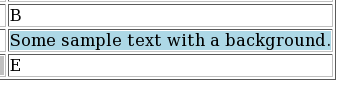
:c.
.*b2h html <div style='background-color: lightblue; display: inline-block;width: 100%;'>
Some sample text with a background.
.*b2h html </div>

In this the c tag is followed by a B2H line to add a div element, with styling. Then we have the actual text to put in the cell. And finally an end div tag.

In this case we set the background colour to a (standard) light blue. The display: inline-block; width: 100% ensures the background colour fills the cell.

The cell looks something like this:

This, of course, can be done at the individual cell level. And it’s easy for a program to generate lines like these new ones.

One nice thing about this technique is you can apply arbitrary CSS to a table cell. For example setting the foreground colour with e.g. color: red;.

Colouring A Heading

It’s perfectly possible to set the format of any heading level. Taking an example from the B2H manual:

.*b2h option headrec.text='<style type="text/css">'
.*b2h option headrec.text='H1    { font-size: x-large; color: red  }'
.*b2h option headrec.text='H2    { font-size: large;   color: blue }'
.*b2h option headrec.text='</style>'

says that all h1 elements will be red. h2 elements will all be blue.

You’d put this at the top of the source.

Colouring Arbitrary Text

In many places in Bookmaster you can use Highlighted Phrases. These are coded somethng like:

Here is some :hp4.highlighted:ehp4. text.

You can define what each highlighted phrase looks like. I’m going to use the example of hp9 which is probably one you’s not normally use. Here’s how you specify its formatting to B2H:

.*b2h symbol :TAG.  HP9 IT=N VAT=N ATT=N SE=Y V='<span style="color: red;">'
.*b2h symbol :TAG.  EHP9 IT=N VAT=N ATT=N SE=Y V='</span>">'
:p.Here is some :hp9.highlighted:ehp9. text.

which formats as:

Conclusion

As I think I’ve shown it’s perfectly easy to enhance Bookmaster source so that when formatted with B2H it adds a dash of colour. More than an em-dash, in fact. 🙂

Now to find places to use it.

(Originally posted 2015-03-22.)

OA37826 really is the gift that keeps on giving: I got really nosy about Coupling Facility links when it came out [1] , though most customers didn’t get the added benefits of CFLEVEL 18 for a while.

This post is about a customer installation which pointed out another benefit of the instrumentation. [2]

Customer Example

I’ve simplified the customer situation a little – in a way that doesn’t detract from the truth. [3]

Here’s a simplified version of their Parallel Sysplex environment:

They have 3 routings between two data centres – and 6 links from each CEC to the CF image in the other data centre. Structure duplexing is not used – as the customer is using external (to this sysplex) coupling facilities.

According to the SMF 74 Subtype 4 data the signalling latency from MVSA to CFB is 161μs (x2), 172μs (x2), and 176μs (x2). You can see the three routes on the diagram.

MVSB shows the same signalling latencies to CFA – which is to be expected.

You’ll notice I’ve used latency – which is what 74–4 gives you. A good rule of thumb is each 10μs of latency translates into 1 kilometer of distance. [4]

I was supplied with the customer’s own diagram and it shows slightly different distances. The discrepancies between the two sets of estimates are not accounted for by any inaccuracy in that formula. I say that because one of the customer’s path distance estimates is substantially lower than my minimum, one if substantially higher, and the third about the same. [5]

It could be a matter of the vendor being inaccurate, though not by much (and life isn’t usually that simple). If the discrepancy was massive compared to this you might begin to suspect “fibre suitcases” left in the route. In any case for once SMF can give you a view of distance.

The “local” latency is 1μs, which is the same as I’ve seen in previous cases. The latency value is an integer number of microseconds and the minimum value is 1 for a supported link type. It means “very short link indeed”.

Both the high values (161 – 176 μs) and the low value (1μs) are consistent with the Adapter types – HCA3-O LR (1X) in the former case and HCA3-O (12X) in the latter. Talking of which, the physical adapters are reported in the Channel Path Data Section (as mentioned in System zEC12 CFLEVEL 18 RMF Instrumentation Improvements ), alongside the latency. So we can see which links / CHPIDs / PCHIDs / ports etc use which routes. [6]

In this customer case there is nothing to recommend. I simply observe the three-route solution, which is patently sensible.

Impact On My Reporting

I’ve modified my reporting only slightly as a result of this customer example, I’m pleased to say.

In my tabular report that documents the paths between z/OS systems and coupling facilities I had one row per z/OS-to-CF pairing. It had the range of latencies for that pairing. In the customer example it said “161 – 176”.

That was useful as it alerted me to the possibility (I hadn’t considered before) of multiple latencies and hence multiple routes. But it told me I could do better:

Now, for each link I list the latency separately – if there is any variation. So, “tourist information” perhaps but I can discuss with a customer their use of alternate routes between sites. [7]

I consider this a nice little piece of (easy to code) extra information.

Final Thoughts

This example shows how you can verify the distance of routes between data centres – or at any rate between z/OS images and distant coupling facilities. You can verify it to within 100 metres, which I think is plenty good enough.

Note that the Coupling Facility does not select paths based on distance/latency. And that latency values are static in all the sets of data I’ve seen. These two facts are mutually consistent.

Also signalling latency is not the same as request service time. It might be interesting to compare latency to service time to try to understand the non-CPU component of service time. But expect Async requests to weaken the correlation – as requests can be expected to be delayed sometimes for reasons unrelated to signalling links.

And finally all this applies equally to links between coupling facilities for structure duplexing.

Anyhow look up the data in your favourite performance reporting tool and try it. You’ll like it!

And wasn’t I naïve when I wrote “Call me nosey [8] but I really want this – as I like to figure out whether machines are close together or in different data centres.” 🙂

(Originally posted 2015-02-21.)

… or probably more.

I was going to use “Send In The Clones” but I’ve already used it – and someone who shall remain nameless once misremembered it as “Let There Be Clones”. Let there be clones, indeed. 🙂

So, how do I detect cloned CICS regions, for example?

(And if you want to know why I’m asking that question now it’s an enforced rereading of CICS XCF Traffic Analysis – A Suitable Case For Treatment to expunge some errors that led me to think about the question.)

In that post I have two CICS regions that appear to behave identically. But that’s just from the XCF Traffic point of view.

What Should Be Similar

Each CICS region’s SMF 30 records will have one or more Usage Data Sections:

• It would be reasonable to expect the CICS section to have the same version and release, though this transitionally might not be the case.
• Similarly, for CICS and MQ, the versions and releases would match, and subsystem names would match. (The subsystem name in this case is consistently embedded in an identifier.)
• For IMS we just get the version and release. But this section’s presence and consistency is to be expected.

Some things should be similar – for well-balanced clones. But see below. Those things include:

• CPU
• I/O rates
• Memory
• XCF traffic, including partner systems.

By “similar” two things to note:

• Exact matches for numeric values are unrealistic.
• Timing is important. The matching would be across all hours of the day.

You might expect restart times and dates to be pretty similar, but these might be rolling – from LPAR to LPAR. And if you dynamically provision cloned CICS regions (not that I’ve ever seen it) the restart times would vary.

Naming conventions are fraught. While clones generally do obey a naming convention more than half of the customers I’ve looked at this way would yield “false positives”. For example CICSA and CICSB are clones, but CICSC isn’t.

What Might Vary

Just because regions are cloned doesn’t mean all the numbers have to match. For example

• If the CICS regions are spread across LPARs (or machines) with different effective engine speeds their CPU times could be expected to vary.
• If work distribution – by whichever method – is uneven a lot of the numbers might vary.
• Memory – whether virtual or real – is quite fraught.

Some Further Thoughts

It’s occurred to me – looking at my current reporting – that some level of clone detection could be automated. To be fair the reporting that puts me on the brink of this is less than a year old. So many reporting ideas; So little time. 🙂

And if I did detect clones, what then? Ideally I’d be generating diagrams. Just yesterday I gave up on drawing a CICS / IMS / MQ / DB2 topology diagram for a sysplex. I gave up because it took too longer to manually gather the data. Actually the diagram layout is the difficult (rather than tedious) bit. But I have ideas… 🙂

As usual, the aim is to get closer to what you’re running and how; And what issues that creates. And I’m a lot further on than I was with He Picks On CICS. The journey continues…

(Originally posted 2015-02-15.)

In He Picks On CICS I mentioned XCF traffic and CICS. This post is about a customer situation where looking at this traffic was important.

Often I’m looking for topology (maybe “tourist information” to some of you). This time I have another motivation: Performance. In this customer saving z/OS CPU is important. [1]

I’ve noticed that the Coupling Facility CPU has XCF signalling structures as a sizeable component. [2] I’ve also noticed that the XCF address spaces [3] on each system consume a lot of CPU.

So the important question is “which XCF groups and members are driving this traffic, and this CPU?”

But we are in “the point, however, is to change it” [4] mode.

So, hard on the heels of the first question is another one: “What conversations between members are driving the traffic”. This question is a prelude to discussions about how to actually reduce the traffic – which is the eventual aim.

Customer Case Study

I’m going to simplify the customer situation without, I hope, any loss of fidelity.

In the sysplex are two intimately-linked systems.[5] Call them SYSA and SYSB. [6]

The major members of the DFHIR000 group on each system are:

• On SYSA is a region I’m calling CICSF. From SMF 30 I can see it does a lot of I/O. From SMF 74–2 I can see a lot of traffic between it and SYSB in group DFHIR000.
• On SYSB are regions I’m calling CICS1, CICS2 and CICS3. These are the ones with the vast majority of the DFHIR000 traffic to SYSA. They also perform very little I/O.

I don’t see much traffic from SYSA or SYSB to other systems in the DFHIR000 group.

The graph below plots, across a day, the traffic for these four members (and it’s genuine, from the data).

We can make the following observations:

• CICSF traffic more or less matches the sum of traffic for CICS1, 2 and 3. But not quite. And it tracks well across the day.
• CICS1 and 3 traffic is pretty evenly matched. So they can be viewed as clones.
• CICS2 has much more traffic than CICS1 and 3. So it’s doing something different. (Or at least more)
• The traffic has peaks at specific times of day. This might be significant.
• The CICS regions don’t go down overnight. [7] They merely slow. [8]

One thing the graph doesn’t show, but the 74–2 data does, is XCF traffic is even in each direction.

So here are some, admittedly tentative, conclusions:

• CICSF is in some sense data owning. The others aren’t.
• CICS1 – 3 ship requests for data to CICSF. The one-to-one ratio of inbound to outbound requests supports that: A request for data followed by the data being returned.
• While the traffic match is pretty good there are probably other CICS regions involved.
• We wouldn’t see requests to CICSF from other regions on SYSA – as they wouldn’t be using XCF.

This Is Not Topology

We can’t claim we’re seeing the whole topology this way, for two reasons:

• The traffic doesn’t entirely match, as the graph shows.
• Traffic from other CICS regions on SYSA to CICSF isn’t detectable.

Yes, these are a restatement. The first one is perhaps resolvable with more processing of the 74–2 data. The second would require different sources of data. Maybe a (guessed) naming convention could help me here. It has before. 🙂

We could, for example, be only seeing part of this topology:

In the above the dashed lines are not XCF. But we could probably guess them just from the existence of regions CICS4, 5, 6 – especially if they behaved like CICS1, 2, 3. [9]

Conclusion

The purpose of this, remember, is to begin to discuss tuning actions that can reduce the XCF traffic between SYSA and SYSB and hence the cost.

I think “begin” is right: Obviously deeper discussions on which region should own the data, for example whether VSAM RLS is the answer, and so on are needed. But at least this is better, I claim, than just saying “try to get DFHIR000 XCF traffic down”.

And note the matching I did is what I call a “guessing game”. It really is. But one day I’d like some code that helps me do the guessing. Maybe I’ll have to build it myself. 🙂

(Originally posted 2015-02-08.)

I have a new conference presentation in mind. Its working title is “DB2 Through My Eyes”. Here’s the structure I’ve devised for it:

• Abstract
• What Is DB2?
• CPU
  • General Purpose
  • zIIP
• Memory
  • Real
  • Virtual
• I/O
  • Database
  • Subsystem
• Application
  • Connections
  • Performance
• Parallel Sysplex
  • Coupling Facility
  • XCF
• Specialist Subjects
  • Restarts
  • Workload Manager
• Stored Procedures
• Conclusion

and here’s a prettier version:

(I made this version with the lovely iThoughts app – on my OSX laptop and my iPhone and iPad – and the text version of the structure was made by exporting to Markdown and some editing in Byword on OSX. I’m experimenting with the workflow.) 🙂

Abstract

Here’s what I have for the abstract right now:

    Bridging the gap in perspectives between DB2 and System Performance specialists is a perennial concern of mine: As a specialist in one you're much more valuable if you CAN bridge that gap.  

    This presentation shows some techniques I use to understand a customer's DB2 environment BEFORE I talk to a customer's DB2 specialists (or indeed my own).  

    All these techniques are available to you, the data being readily available. I hope you find them useful.

Conclusion

I think I have material that covers the ground, but I’m open to ideas. I suppose I have the advantage here as I have some thoughts about what each of these topics really boils down to. There are several months to go before I actually have to turn the slides in – but that might be less time than I suppose as I’ve already had one offer of a user group appearance.

As you probably know I like to introduce at least one new presentation a year. (Last year I did two and maybe I will again this year: The year is still young.)

And I’m playing with the idea: “This is a bridge, not a bypass.” By this I mean this enables System Performance specialists and the like to talk to DB2 people better, rather than attempting to circumvent them.

And “stay tuned” for any “design in public work” on this. There’s quite likely to be some.

(Originally posted 2015-01-10.)

As I’m working with a couple of colleagues on a performance study I thought I’d list some “starter set” questions I’d ask about any customer’s WLM policy.[1]

Before you go too far with this post you might like to read Analysing A WLM Policy – Part 1 and Analysing A WLM Policy – Part 2 but I don’t think I’m repeating myself much here.

So here are some key questions I can seek to answer:

• Does the policy have a reasonable Importance distribution, CPU-wise?[2]
• Is work appropriately classified?[3]
• Are Importance 1 goals met barely, easily, or not at all?
  • How do they bear up with load?
  • Which components of Using and Delay feature most highly?
• Are Importance 2 goal met barely, easily, or not at all?[4]
• Do transaction-based goals have the right kind of period structure?
• Does the policy have a proliferation of active service class periods?
• Is there a sensible separation between velocity levels?[5]
• Are policies enabled effectively?[6]
• How are Report Classes used?

Many of you, I’m quite sure, are capable of answering all these questions – based on your analysis of your own data. But certainly these are questions I’m likely to address if you’re one of the customers I’m lucky enough to deal with.[7] Indeed I wrote a slide of questions – you might see – in parallel with writing this post.

Food for thought? 🙂

And one final thought: There’s a question I can’t directly answer but would work with any customer of mine on:

• How do the goals relate to business goals? For example, “where did this Response Time goal come from?”

(Originally posted 2014-12-31.)

It’s a little surprising to me that nobody complained about one aspect of the behaviour in the code in GreaseMonkey Script To Sum Selected Numbers In A Web Page. I’ve been muttering under my breath and I wrote the code. 🙂

This code naively assumes that in every web page there is just one body element. It is rather naive, and I’ve known that for a long time.

What really surprised me was quite how prevalent multiple body elements are in a page. Yes, I expect that in frames; no I don’t expect too many other cases.

So, I’ve been noticing lots of pages where the little “Sum Up” button showed up in places I didn’t expect it; It seems people embed body elements in all sorts of strange places.

The fix is really very simple. I’ll show you it and then I’ll explain it.

So replace the lines

    // @version     0.0
    // ==/UserScript==

with

    // @version     0.1
    // ==/UserScript==

    // Only add to topmost window in the tab
    if(window.top!=window.self) return

and now the script will only add the button at the top of the page / tab.

So the magic here is in knowing window.top is the top-most window in a web page. The script is loaded in every window – but this new line says "do nothing for every window that isn’t the topmost window.

Now, what’s (only slightly) surprising is that nobody’s complained. It probably means only one thing: Very few people have installed the script.

But I have – and I’m benefiting from it. So I’m still ahead.

And with that I’ll wish you all a Happy New Year! (Conscious as I am that for some the new year starts at a different time but deeming it much less controversial than “Merry Christmas”. If you wish me a Happy or Merry anything I’ll probably say “thank you very much and the same to you”. “War On Christmas” my eye!)

(Originally posted 2014-12-13.)

This post is meant to inspire people who like programming the web to do simple tasks. It contains a sample Firefox GreaseMonkey [1] script, which I hope you will find useful. [2]

Suppose you are looking at a web page, perhaps one with a table in, and you want to add up some numbers you see there. Perhaps they’re in a column in that table.

With this script you select the numbers you’re interested it and push the “Sum Up” button that appears at the top.

Here’s the script:

    // ==UserScript==
    // @name        swipeCalc
    // @namespace   MGLP
    // @description Does calculations on selected text
    // @version     0.0
    // ==/UserScript==

    input=document.createElement("input")
    input.type="button";
    input.value="Sum Up";
    input.onclick = showResult;
    document.body.insertBefore(input,document.body.firstChild)

    function showResult()
    {
      // Get array of space- and range-separated tokens
        selection=window.getSelection()
        var tokens=[]
        for(r=0;r<selection.rangeCount;r++){
            rangeTokens=selection.getRangeAt(r).toString().split(" ")
            for(t=0;t<rangeTokens.length;t++){
                tokens.push(rangeTokens[t])
            }
        }

        // Sum up any detected number values
        tally=0
        count=0
        maximum=Math.max()
        minimum=Math.min()
        for(t=0;t<tokens.length;t++){
            tokenValue=parseFloat(tokens[t])
            if(!isNaN(tokenValue)){
                tally+=tokenValue
                count++
                maximum=Math.max(maximum,tokenValue)
                minimum=Math.min(minimum,tokenValue)
            }
        }
        alert("Sum: "+tally+" Average: "+tally/count+" Minimum: "+minimum+" Maximum: "+maximum)
    }

Everything up to the function definition is code to insert a button at the top of every page, with the words “Sum Up” on it. [3] When you push the button it invokes the function “showResult”

Most of the code is the function “showResult”, which is actually quite simple:

• First we break up the (perhaps disjoint) selected text into words.
• Then we loop through all the tokens, using parseFloat() to turn them into floating-point numbers. [4]

• For each valid floating point we use it to contribute to the sum, average, maximum and minimum tallies.
• We display in an alert the statistics we’ve computed.

I hope this script doesn’t look intimidating. Personally I intend to build on it – as there’s so much more we can do with GreaseMonkey.

When I wrote about GreaseMonkey in 2005 I didn’t then realise I’d be using it to prototype Firefox Extensions. I just might do that here. But, of course, time is fleeting and there are lots of challenges out there, with more appearing (it seems) every day.

(Originally posted 2014-12-07.)

I thought I’d write about how I begin looking at virtual storage, occasioned by a customer who had a 24-bit virtual storage (878–10) ABEND[1] . Most of this is in our code, so easy for me to do. I hope you’ll find it similarly easy.

You’ve had hints of this in How Many Eggs In Which Baskets? and Broker And SMF 30.

The game is really to use product-neutral instrumentation first. Then use the product-specific instrumentation (where available) only where you really need it.

This post won’t talk about the latter; It’s reasonably well documented.

Almost everything I’m about to say is equally true of 24-bit and 31-bit virtual storage; Just the field names are different in the records.

I divide the analysis into two parts:

• System Virtual Storage
• Address Space Virtual Storage

The data for the former comes entirely from RMF’s SMF Type 78 Subtype 2. For the latter it’s in the SMF Type 30 record (though you can also get SMF 78–2 information for a small number of suitably-chosen specific address spaces.

System Virtual Storage

Here we establish how the Common areas are defined and used, together with the size of the Private area.

This is easy to do. In this example the data is all 24 Bit.

The highest level view looks like this:

This is a static picture.

The first thing to notice is that the Common Boundary is at 9MB.[2]

In case you need a larger Private Area examine the largest allocated area of Common Storage and it is, in this case, CSA.[3]

Here’s how I begin to drill down into CSA usage (rather than allocation):

(You might want to pop it out into a different tab – as it’s quite wide.)

Each line, except the first two, represents a different time range. In this case I’m summarising at the half-hourly level. [4]

The first two lines are maxima and minima. In this case they show only slight variation through the day, which is good to know.

The first thing I notice about this is there is some SQA free (and in the 31-bit case I print a “SQA Overflow Into CSA” column instead – as that’s what’s happening with this set of data). SQA can overflow into CSA but not vice versa – so this is wasted virtual. I recommended decreasing the SQA size by, say, 250KB [5]

That’s not strictly necessary as the Minimum CSA free (rightmost column) is over 2.5MB. So an easy way to get a 10MB region is to decrease the CSA size by 1MB. 2MB would be pushing it – as the customer wants to allow the whole of Key 7 to be duplicated. [6]

Talking of which, you can work out which Storage Protection Keys represent the bulk of the CSA usage. In this case it’s Key 0, Key 7 and Key 8+. [7]

But you can go further. Look at this:

It’s Subpool 241 Key 0 that’s the biggest, then Subpool 228 for Key 8+, then evenly split Subpools 231 and 241 for Key 7.

I’ve deliberately summarised this table over a “shift” – to avoid having to make the table 3-dimensional 🙂 . But the conclusion is still clear.

If you had to tune CSA usage you’d use this information and drill down further.

For completeness, here’s the Subpool breakdown for SQA:

It’s obvious Subpool 245 dominates.

Two things to note:

• You don’t get either the CSA or the SQA Subpool breakdown for 31-bit (as it’s not in the data).

• You can’t break down the SQA Subpool usage by Storage Protection Key.

But you can see a good breakdown of Common Storage can be had from RMF 78–2 data.

Fortunately, we can already do enough with just a CSA reduction (and perhaps with a SQA reduction) to get us at least 1MB more 24-bit Private.

Address Space Virtual Storage

Here we examine Private Area Allocated [8] Virtual Storage for individual address spaces.

While it’s possible to examine Private Area virtual storage with SMF 78 Subtype 2 data most customers don’t set up monitoring of individual address spaces.

Instead SMF 30 Interval records tend to be readily available. So from these you can get 24- and 31-Bit “Low Private” and “High Private” numbers.

In the example customer’s case their IMS DL/I SAS (address space) takes almost the whole of the 24-bit Private Area. About half is Low Private and half is High Private.[9]

Interval-on-interval there is little change is Private Area usage (but I don’t have data from the day the ABEND happened – yet). It’s just clear this address space is always “close to the edge”.

So, working on the 24-bit virtual storage usage by this address space is strongly indicated. But having a 1MB bigger 24-bit region can’t hurt either. So I’ve advised doing both.

Conclusion

I hope you can see it’s quite easy to analyse virtual storage with SMF 78–2 and SMF 30 Interval records.

I’d say that – with a few exceptions – you shouldn’t obsess over virtual storage. What you should do is consider setting up some “light touch” monitoring; Perhaps CSA Free and SQA Free (24- and 31-bit) and Virtual Allocated for some key address spaces. That way the usual applies:

• You get to know how your systems operate.
• You can spot impending problems.

And I’m going to make sure in future we always pump out this sort of reporting – assuming the data’s there. And generally it is: You’re collecting it so use it.